DOI:10.28974/idojaras.2019.3.2
IDŐJÁRÁS
Quarterly Journal of the Hungarian Meteorological Service Vol. 123, No. 3, July – September, 2019, pp. 279–294
Supporting microclimate modeling with 3D UAS data acquisition
Zsófia Kugler 1, Zoltán Tóth 2, Zsuzsa Szalay 3, Dóra Szagri 3, and Árpád Barsi *,1
1 Department of Photogrammetry and Geoinformatics Budapest University of Technology and Economics
Műegyetem rkp. 3, H-1111, Budapest, Hungary
2 Institute of Geoinformatics, Óbuda University Bécsi út 96/B, 1034 Budapest, Hungary
3 Department of Construction Materials and Technologies Budapest University of Technology and Economics
Műegyetem rkp. 3, H-1111, Budapest, Hungary
*Corresponding author E-mail:barsi.arpad@epito.bme.hu (Manuscript received in final form June 3, 2019)
Abstract⎯ Microclimatic analysis of an urban scenario has always been an interesting but complicated challenge. The available remote sensing equipments ensure multi- or hyperspectral imagery being ready to extract excellent land cover information, but the obtained data have lower spatial resolution limiting the efficiency of such analyses. In order to increase the geometric resolution in microclimatic studies, an exercise was executed with an Unmanned Aerial System. The calibration of the imaging camera on a dedicated test field was followed by the data capture flight over the campus of the Budapest University of Technology and Economics. The evaluation of the acquired images has resulted a point cloud containing millions of points. The high density point cloud was able to be transformed into 3D mesh representation and could be fed into a geographic information system for further analysis steps. Based on the color and height information of all individual points, the obtained geometric base was easily to be converted into land cover model representing man-made and natural objects, like buildings or trees. The segmentation of the model is a suitable input for climatic analyses and simulation software packages, where extreme high geometric resolution is required.
Key-words: urban microclimate, building heat balance, UAS, camera calibration, 3D surface model, canopy structure
1. Introduction
A microclimate is the distinctive climate of a small area, such as a garden, park, valley, or part of a city. The weather variables in a microclimate may be subtly different to the conditions prevailing over the area as a whole. While a particular climate is representative for a large area over long periods of time, microclimate refers to a climate over a very small area. Local conditions can alter climate, for example the presence of vegetation causes cooler and wetter microclimate in its surroundings. Typical microclimate environments are urban regions, where the presence of anthropogenic activity and build-up environment may alter weather conditions compared to its surroundings. Since urban expansion has been facing an exponential rise during the last century, urban microclimate is a target of investigations for decades.
It has been observed that urban areas are generally warmer than its surrounding rural environment (Barry et al., 2016). This phenomenon is called the Urban Heat Island (UHI) effect. Multiple factors like change in surface materials, lack of evapotranspiration, urban canyon effect, and anthropogenic heat release may cause the formation of UHIs (Liang et al., 2012). According to the Met Office Factsheet (MOF, 2019), in the UK, temperature contrast of urban (London) and rural areas was found to be up to 5 °C on in mid-May during clear sky conditions. Climate change is expected to exacerbate the UHI effect, increasing the cooling energy consumption and also severely affecting human health. Understanding and analyzing urban microclimate, evaluating UHI effect and heatwave vulnerability is particularly important for urban public planning measures.
For this reason, urban planning, urban landscape design, and emergency services should obtain a clear understanding of the phenomenon in order to plan sustainable measure and mitigation strategies for the current and future situations.
Urban microclimate characteristics are difficult to measure, since the sampling density of in-situ meteorological stations are usually not dense enough to reveal spatial distribution of local weather parameters. To set an example in Budapest (Hungary) which is a capital of almost 2 million inhabitants on 525 km2, only 4 meteorological observation stations are in operation and not all situated in standard measuring environment. Hence to study urban effects on local climate, asses risk, and resilience of urban population related to heatwaves, microclimate has to be expressed using simulations, modeling supported by indirect measures.
2. Remote sensing to support microclimate models
Thermal remote sensing technology has been successfully applied in microclimate observations of urban temperature patterns. The first satellite-based analysis of an urban heat island was performed by P. K. Rao (Rao, 1972), which was followed by numerous studies in the past decades. Both satellite and aerial platforms were
applied to perform observations on Land Surface Temperature (LST) to map UHI.
Thermal infrared (TIR) satellite sensors of MODIS, Landsat, AVHRR, ASTER, ATSR, SEVIRI, HCMM were extensively used in LST retrieval (Zhou et al., 2019). Besides, airborne data also offers numerous advantages and has been used in urban thermal heat mapping. Yet both acquisition platforms are not necessarily following the spatial, temporal, and spectral resolution needs of the application.
In order to analyze urban climate, Unmanned Aerial Systems (UAS) with high resolution imaging capabilities offer a good solution. Due to the local scale characteristic of local urban climate, the small scale acquisition techniques of UAS remote sensing can better meets the objectives than satellite or aerial remote sensing. Compared to satellite images, the advantage of using UAS is in the temporal frequency or high repetition rate of the recordings. Using thermal UAS sensors, daily dynamics of small scale thermal variations can be easily measured by repeated flights during a given day. UAS is appropriate to estimate surface microclimate indicators by low cost acquisition and processing compared to aerial data capturing (Kotchi et al., 2016). UAS not only has the advantage of local scale data acquisition but also the repetition cycle is not limiting factor in temporal density of observations. What is more, image capturing is not limited to cloud- free weather conditions.
Therefore, a study has been carried out how optical UAS sensors can collect valuable information to support urban microclimate modeling and building energy simulations. Besides 3D surface modeling, different types of local scale characteristics of urban land cover were derived too. The study has been dedicated to understand what type of parameters can be derived particularly on urban vegetation cover not only from nadir looking but from oblique UAS acquisition techniques to support microclimate modeling. Future plan is to analyze the outdoor building heat conditions by thermal UAS measures captured during summer season to better understand and simulate in-door thermal conditions during heatwaves.
Microclimate is primarily depending on the surface albedo of a given object, which expresses the ratio of reflected sunlight to irradiance. Several field and laboratory measurements are able to determine albedo (Chen et al., 2019). With the latest technology, an accurate and high resolution albedo can be derived using a combination of a digital camera, broadband pyranometers, and UAS platform (Ryan et al., 2017). With this technique, the effect of large trees on microclimate can be evaluated properly (Eckmann et al., 2018), which could lead to better decisions in urban planning. According to the latest research, the changes in surface temperature depend on the albedo and apparent thermal inertia (Gaitani et al., 2017a).
Vegetation cover is very important for reducing the ambient air temperature.
Based on measurements, the temperature difference between a dense green area and a built-up university campus residence may reach 4 °C on a summer day (Wong et al., 2007). By combining on-site measurements and numerical
simulations, we can get accurate results showing how to improve the microclimate of a given area using green surfaces (Srivanit and Hokao, 2013). In the case of community spaces (campuses, playgrounds, town squares etc.), it is important to assist decision makers, since large population are exposed to thermal stress, which is mainly influenced by the design of the landscape zone (Égerházi et al., 2013).
To map vegetation activity of a given area, NDVI (Normalized Difference Vegetation Index) can be derived from near infrared (NIR) images (Gaitani et al., 2017b). This value quantifies the vegetation by measuring the difference between near infrared (NIR) and visible red (RED) bands, and the results can be used when making microclimatic design decisions. 3D oblique viewing UAS data acquisition can derive information beyond this. Vegetation surveys together with 3D canopy surface can be efficiently conducted, even over moderately large areas (Cruzan et al., 2016).
The use of UAS in microclimate analysis can be a useful tool even without special sensors, as image processing can deliver input data for building heights and vegetation in several simulation models.
In the future, urban land use will change along with the population’s age and structure patterns. By examining different future scenarios, development of new urban areas was projected in Hungary to be mainly around the capital and regional centers (Li et al., 2017), therefore, the analysis of urban environment and microclimate needs to be at the forefront of research.
2.1. UAS-based imaging technology
Vehicles of the Unmanned Aerial Systems can be grouped into two main clusters:
the fix wing and the rotary wing systems. Fix wing vehicles have high similarity with airplanes, while rotary wing vehicles with the helicopters. In our research we have conducted all field works with a rotary wing system. Depending on the number of rotating wings (the rotors), one can speak about quadrocopters (with 4 rotors), hexacopters (with 6 rotors), or octocopters (with 8 rotors). There are high variety of rotor configurations.
The system consists of the flying vehicle (Unmanned Aerial Vehicle – UAV), a ground based controller, and a communication system. The vehicle is a platform carrying the navigation and control, as well as the imaging equipment.
Navigation system is responsible for serving information about the current position of the vehicle and specifying the commands for the motors. Control component affects the behavior of the vehicle’s engines by increasing or decreasing the revolution rate individually. The imaging system is the most important payload component: it is for capturing the data, in this case the images.
The ground based part of the system is a device, where the pilot can control the flight of the vehicle, start or stop the image streams, and receives all data coming from the vehicle. Therefore, UAS is also called as Remotely Piloted Aerial System (RPAS). Communication solution is for transferring data and
commands between the ground and the flying component. Both the ground controller and the vehicle are equipped with suitable power supply.
UAS has different degrees of autonomy: pilots have to react for all circumstances (wind, vibrations, etc.), there is a functionality to stabilize the vehicles, it gets prior the flying and image capturing instructions and executes them. This last option is a kind of automated flight, which is very advantageous in field survey tasks.
The workflow (Fig. 1) starts with mission planning, where the boundary of area to be surveyed must be exactly set, then a flying plan has to be elaborated considering the features of the aerial vehicle. There is a bunch of commercial and freely available software tools to support the mission planning.
Fig. 1. The general UAS workflow.
The planned flying trajectory and commands must be transferred onto the vehicle, and after take-off, it can be instructed to go alone. Under continuous human control the flying vehicle executes the image capture task and obtains the required data set. GNSS measurements (like GPS with e.g., Real Time Kinematic measurement modus, RTK) can define ground control points (GCPs), which have mapping coordinates and can be identified in the obtained imagery. Prior point marking with colored plates can increase the available computational accuracy.
The data processing starts with downloading the images and entering a photogrammetric evaluation software. The image processing software of nowadays have a strong base on computer vision principles; the driving methodology is mostly the Structure-from-Motion (SfM) technique. The algorithm defines well-identifiable points in all images; this is the interest operator phase. Thousands of image observations have to be paired in all combinations, but only those are kept, which exceed a preliminary limit of correspondence. By the use of corresponding points, the projection centers and orientation angles are calculated for each captured image. A sophisticated bundle block adjustment can minimalize the overall matching errors and creates a basic geometric model.
Having all images oriented, the multi-view stereo (MVS) algorithms evaluate the images. This step will result a dense point cloud of the interest area.
This phase requires the most computation power. After getting millions or even billions of object points, the obtained point cloud must be complemented with regular topology, like a triangle network, so a mesh model can be achieved. Mesh
triangles can be extended by the color information of the original images. A colored point mesh is the base of all photorealistic visualizations. In Geographic Information System (GIS) applications, the obtained point clouds and mesh models are used as Digital Surface Models (DSM) and Digital Elevation Models (DEM), as filtering and similar techniques can differentiate between the bare Earth height information and covered natural (typically the vegetation) and human objects (buildings, roads, etc.). DSMs and DEMs can be later used in form of terrain sections. The work is usually finished by deriving an orthoimage mosaic.
2.2. Calibration of UAV cameras
An important processing step in both the aerial photogrammetry (used for mapping purposes) and close range photogrammetry (used mostly for object reconstruction) is to determine the internal and external orientation parameters.
The internal orientation data consists of the principal point coordinates and the focal length. The image coordinate system is determined by the array of pixels.
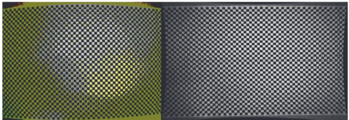
Another parameter having significant impact on the metric quality of an image is the lens distortion. In general, low cost lenses are expected to have significantly higher distortions compared to lenses of professional metric cameras. There are many software packages available for deriving the interior orientation parameters (including the lens distortion). Usually, the calibration procedure has been done automatically using imagery of black-and-white (B&W) checkerboard targets (Fig. 2).
Fig. 2. B&W checkerboard calibration target before and after applying the calibration.
The exterior orientation parameters ensure the transformation between the image coordinate system and the mapping (or object reconstruction) coordinate system: three parameters for translation (x, y, z) and three for Eulerian rotation angles (omega, fi, kappa). It is possible to measure (usually preliminary) exterior orientation parameters with GNSS and IMU sensors. Final parameters are usually computed by using aerial triangulation (AT) process based on ground control points (GCP) with known mapping coordinates. For more efficient workflow and
more accurate results it is very common to combine these two methods, involving GNSS and IMU observations together with GCPs in an AT process. It is very common in today’s practice, that the interior and exterior orientation parameters are determined in one single processing session. Due to the highly automated processing workflow, many software packages give the users very limited freedom of control over the calculation parameters. These black-box-like solutions are getting more common thanks to the growing popularity of UAS based mapping systems.
Since the spatial accuracy of many mapping projects must meet a certain threshold given by governmental standards, by the customer, or simply by the nature of the project, the quality of the end product must be proven and well documented. A black-box-like processing workflow is not able to meet this requirement. To address this issue, the Alba Regia Faculty of Óbuda University created a test and calibration site for UAS based mapping systems. The high quality, high accuracy test site has been created for system calibration, reliability investigations, and performance analyses.
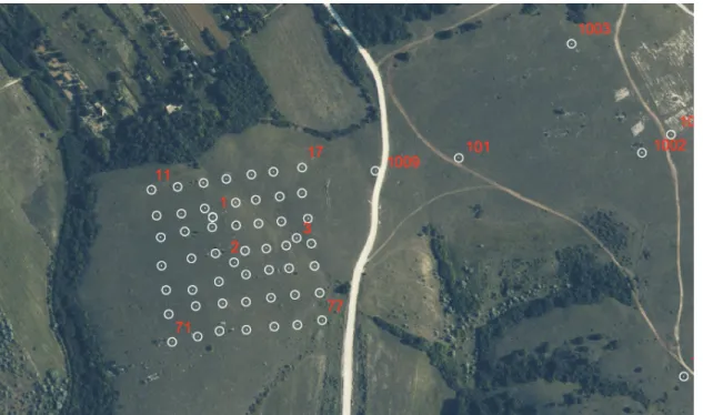
Fig. 3 shows this 200 m × 200 m sized test field on a hilly terrain. The 7 × 7 array of GCPs is roughly oriented to North. The terrain consists of relatively even areas as well steep hillsides. The maximum difference in elevation is approximately 20 meters.
Prior to our investigation on the BME campus, the applied UAS camera has been calibrated in the test field, and the obtained parameters are kept for the later computations.
Fig. 3. Calibration test field near Székesfehérvár.
2.3. UAS survey on BME campus
The applied UAS was a DJI Phantom 4 system. The flying vehicle (Fig. 4a) has been equipped with a synchronous image transfer (first person view – FPV) option that forwards the current flying parameters (e.g., height, speed, tilt, power reserve), too.
Our study area is the northern and middle campus of BME. In order to get homogeneous geometric accuracy, we have decided to execute the flight in fully automated mode in double grid formation (Fig. 4b). There were six ground control points installed with red and white colored 1 × 1 m size plastic plates (Fig. 4c).
The center of the GCPs were measured by a Leica CS10 GNSS receiver. The measurement was done in RTK mode supported by the Hungarian RTK network.
The vehicle is equipped with a camera mounted onto a 2 DoF gimbal. The camera has a fix focus lens of 2.77 mm focal length and is capable to acquire image with 3000×4000 pixels. The stored image format was sRGB jpg, the sensitivity was set to ISO 100. The aperture was also fixed for 2.8, while the shutter speed was varied to adjust the exposure adequately. Generally, the shutter speed was set to 1/400 s.
The mission was executed in the morning between 9:00 and 12:00, on April 1, 2017, the flying time was about 32 minutes for the northern and about 28 minutes for the middle campus. The overall flying time was 1 hour. There were 489 images taken in the northern and 429 in the middle campus. The total number of images is 918. The required storage capacity was 2.75 GB. The compression rate is better than 1:10 in average.
The photogrammetric image processing was done with the Pix4D Mapper software, which is available also as cloud service. The available performance is scalable, after uploading the image and GNSS data into the cloud, the following computing power was given: Intel Xeon CPU E5-2666 v3 @ 2.90GHz CPU with 59GB RAM and Cirrus Logic GD 5446 GPU. The operating system behind the computations was Linux 3.13.0-91-generic x86_64.
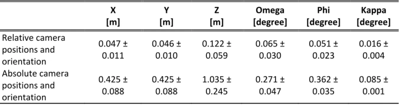
The applied software has used SfM based technology also. The parameters from the test field calibration were also uploaded. The bundle block adjustment was initiated by 7 125 323 points, then the results of the orientation can be summarized in Table 1.
a) The DJI Phantom 4 drone in work
b) The planned mission with the double grid imaging
c) Installation of a ground control point Fig. 4. The image caption technology with DJI system
Table 1. Relative and absolute camera positions and orientation parameters with accuracy measures after bundle block adjustment
X [m]
Y [m]
Z [m]
Omega [degree]
Phi [degree]
Kappa [degree]
Relative camera positions and orientation
0.047 ± 0.011
0.046 ± 0.010
0.122 ± 0.059
0.065 ± 0.030
0.051 ± 0.023
0.016 ± 0.004 Absolute camera
positions and orientation
0.425 ± 0.088
0.425 ± 0.088
1.035 ± 0.245
0.271 ± 0.047
0.362 ± 0.035
0.085 ± 0.001
The computation time for the complete orientation with bundle block adjustment was 1 hour 19 minutes.
These more than 7 million points are only a sparse representation of the interest area. The higher quality dense point cloud has been achieved after 44 minutes computation. The dense point cloud contains 55 797 678 points with RGB color information, which means a spatial point density of 71.98 points/m3. Based on the point cloud, a mesh model was also derived after 23 minutes run.
The obtained mesh model has been built with 1 million triangle elements. The point cloud can be visualized with sophisticated GIS tools, like QGIS as in Fig. 5.
Mesh means a photorealistic visualization, see Fig. 6.
Fig. 5. Plastic visualization of point cloud in QGIS.
Fig. 6. Perspective view of mesh model (it is a composite view of 1 million colored triangles).
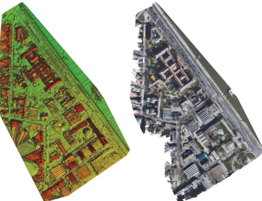
The point cloud serves as a base for computing regular Digital Surface Model (DSM) and an orthoimage mosaic (Fig. 7). Our interest area of the university campus has an extent 600.5, 871.3, and 79.1 m in X, Y, and Z directions, respectively. The suggested ground sampling distance was 3.27 cm, whereas the total covered area took 28.53 ha. The production of DSM and orthomosaic took further 13 and 30 minutes computation.
Fig. 7. False-color Digital Surface Model and orthophoto mosaic for the covered area.
2.4. Vegetation mapping from UAV imagery
Having a closer look on the DSM, one can realize that the building and tree heights can be differentiated by some threshold operations (Fig. 8). Trees are typically irregular circular blobs having less heights than the regularly built buildings.
Fig. 8. False-color visualization of the heights of the DSM (same detail as in Fig. 5)
The land cover categories (building, road, grass, tree) can be estimated by the pixel color of the orthoimage, still some manual inspection and fixing is required.
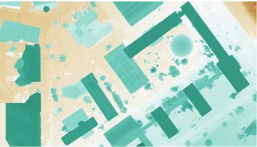
After some manual correction of the differentiation, the vegetation map has been achieved (Fig. 9).
Fig. 9. Vegetation map for the northern campus.
3. Climatic analyses
Urban microclimate is controlled by many parameters, not only by the albedo of the surface. Both natural and man-made elements in the urban landscape interact resulting in a complex response to solar energy gain. Microclimate is not only controlled by building materials and outdoor surface materials of the built-up environment but the presence of vegetation is principally influencing radiation fluxes. Building energy exchange is not only influenced by air temperature but a major impact is dedicated to outdoor vegetation cover.
The effect of vegetation cover on microclimate is enormous. Not only evapotranspiration but also shading plays a key role in influencing urban heat transfer. The cooling effect of vegetation presence is important. Besides, air quality can also be influenced by trees altering the distribution of pollutants in field. For this reason, the detailed mapping of large scale vegetation cover and vegetation structure like canopy distribution can improve the urban microclimate models.
Nadir viewing optical remote sensing sensors can only obtain information like vegetation cover, type or leaf area index (LAI) in general. Only the latter responds to the demand to deduct information over canopy structure. On the contrary, oblique viewing UAS optical data can gather information on the canopy surface resulting in more detailed information on vegetation pattern.
Parameters of canopy volume and structure can support urban microclimate models like ENVI_met or building heat balance-based energy simulation like Energy Plus.
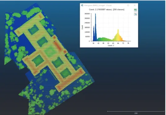
From nadir viewing UAS images, it is possible to capture and derive vegetation extent maps (Fig. 9). However, using the oblique viewing capability of UAS acquisition, the vertical surface of vegetation around the buildings was captured during the study. Therefore, vegetation extent information can be extended with data on canopy structure. In a first step, vegetation was derived from DSM data by histogram thresholding (Fig. 10). A clear distinguish could be achieved by defining grassland below 40 m, trees between 40 and 58 m, and roof was established for all points above 58 m. This segmentation process leads to a clear difference between trees and grassland of the campus land cover classes.
Fig. 10. Vegetation map for the northern campus by DSM histogram thresholding.
In a next step, DSM data over area covered by trees on grassland was studied in more details to support microclimate simulations (Fig. 11). The height of individual trees can be deducted from its surface model. Furthermore, the canopy is clearly distinguishable from tree-trunk, thus a ratio of these two characteristic geometric parameters can be derived from the DSM model. Canopy geometry can help to estimate canopy volume which can be highly correlated to LAI for a given tree type. Geometric properties of tree canopy surface can support both shading calculations and tree evapotranspiration estimates to calculate local cooling effects. Once tree types are derived, predefined phenologic annual lifecycles of plants can be simulated in microclimate models too.
Fig. 11. Tree canopy surface model as height shading (left) and perspective true-color view (right).
Another major influence of urban microclimate is geometric parameters from built-up environment like building height. DSM can help to measure on building height, roof structure, window size, or even shading elements on the building facade. All these parameters influence in-door thermal conditions in a building and can support calculations of building energy balance.
4. Conclusion
The Unmanned Aerial Systems are flexible, easy-to-use image data capture technique, which has already been proven in several technical aspects. Its capability to create high resolution geometric models of urban scenarios enables it to be involved also in microclimatic analyses and simulations. The freely adjustable flying height considering the camera resolution allows to obtain geometric models with prior designed information content. Beyond the pure geometry of the focus area (with building blocks, road surfaces, etc.), such elements can also be described which affect the microclimatic circumstances as the vegetation. Trees, bushes, and grass surfaces can be identified by manual to (semi)automatic techniques based on color and height information. After the segmentation the parameters of the vegetation like tree heights, types, canopy volumes, etc., can be extracted, being able to transfer them into sophisticated climatic modeling software environment. Thanks to the mobility of the UAS technique and the corresponding data processing workflow, the data acquisition demand of microclimatic research has got a new powerful aid.
Acknowledgement: The research reported in this paper was supported by the Higher Education Excellence Program of the Ministry of Human Capacities in the frame of the Artificial Intelligence Smart City (BME FIKP-MI/SC) and Water sciences & Disaster Prevention (BME FIKP-VÍZ) research areas of BME.
References
Barry, R.G. and Blanken, P.D., 2016: Microclimate and Local Climate. Cambridge University Press.
https://doi.org/10.1017/CBO9781316535981
Chen, J., Zhou, Z., Wu, J., Hou, S., and Liu, M., 2019: Field and laboratory measurement of albedo and heat transfer for pavement materials, Constr. Build. Materials 202, 46–57.
https://doi.org/10.1016/j.conbuildmat.2019.01.028
Cruzan, M.B., Weinstein, B.G., Grasty, M.R., Kohrn, B.F., Hendrickson, E.C., Arredondo, T.M., and Thompson, P.G. 2016: Small Unmanned Aerial Vehicles (Micro-Uavs, Drones) in Plant Ecology, Appl. Plant Sci. 4(9). https://doi.org/10.3732/apps.1600041
Eckmann, T., Morach, A., Hamilton, M., Walker, J., Simpson, L., Lower, S., McNamee, A., Haripriyan, A., Castillo, D., Grandy, S., and Kessi, A. 2018: Measuring and modeling microclimate impacts of Sequoiadendron giganteum, Sust. Cities Soc. 38, 509–525.
https://doi.org/10.1016/j.scs.2017.12.028
Égerházi, L.A., Kovács, A., and Unger, J., 2013: Application of microclimate modelling and onsite survey in planning practice related to an urban micro-environment, Adv. Meteorol. 2013, Article ID 251586. https://doi.org/10.1155/2013/251586
Gaitani, N., Burud, I., Thiis, T., and Santamouris, M., 2017a: High-resolution spectral mapping of urban thermal properties with Unmanned Aerial Vehicles. Build. Environ. 121, 215–224.
https://doi.org/10.1016/j.buildenv.2017.05.027
Gaitani, N., Burud, I., Thiis, T., and Santamouris, M., 2017b: Aerial Survey and In-situ Measurements of Materials and Vegetation in the Urban Fabric. Proc. Engineer. 180, 1335–1344.
https://doi.org/10.1016/j.proeng.2017.04.296
Kotchi, S.O., Barrette, N., Viau, A.A., Jang, J., and Gond, V., 2016: Estimation and Uncertainty Assessment of Surface Microclimate Indicators at Local Scale Using Airborne Infrared Thermography and Multispectral Imagery. In (Eds. Imperatore, P. and Pepe, A.) Geospatial Technology - Environmental and Social Applications. IntechOpen, 574–643.
https://doi.org/10.5772/64527
Li, S., Juhász-Horváth, L., Pedde, S., Pintér, L., Rounsevell, M.D.A., and Harrison, P.A., 2017:
Integrated modelling of urban spatial development under uncertain climate futures: A case study in Hungary. Environ. Modell. Software 96, 251–264.
https://doi.org/10.1016/j.envsoft.2017.07.005
Liang, S., Li, X., and Wang, J., 2012: Advanced Remote Sensing: Terrestrial Information Extraction and Applications, Academic Press.
Met Office Factsheet, 2019: https://www.metoffice.gov.uk/research/collaboration/ukcp/factsheets, Last access: 2019-02-22.
Rao, P.K., 1972: Remote sensing of urban heat islands from an environmental satellite. Bull. Amer.
Meteorol. Soc. 53, 647–648.
Ryan, J.C., Hubbard, A., Box, J.E., Brough, S., Cameron, K., Cook, J.M., Cooper, M., Doyle, S.H., Edwards, A., Holt, T., Irvine-Fynn, T., Jones, C., Pitcher, L.H., Rennermalm, A.K., Smith, L.C., Stibal, M., and Snooke, N., 2017: Derivation of High Spatial Resolution Albedo from UAV Digital Imagery: Application over the Greenland Ice Sheet. Front. Earth Sci. 5, 40.
https://doi.org/10.3389/feart.2017.00040
Srivanit, M. and Hokao, K., 2013: Evaluating the cooling effects of greening for improving the outdoor thermal environment at an institutional campus in the summer. Build. Environ. 66, 158–172.
https://doi.org/10.1016/j.buildenv.2013.04.012
Wong, N.H., Kardinal, S.J., La Win, A.A., Kyaw Thu, W., Syatia Negara, T., and Xuchao, W., 2007:
Environmental study of the impact of greenery in an institutional campus in the tropics. Build.
Environ. 42, 2949–2970. https://doi.org/10.1016/j.buildenv.2006.06.004
Zhou, D., Xiao, J., Bonafoni, S., Berger, C., Deilami, K., Zhou, Y., Frolking, S., Yao, R., Qiao, Z., and Sobrino, J.A., 2019: Satellite Remote Sensing of Surface Urban Heat Islands: Progress, Challenges, and Perspectives. Remote Sensing 11, 48. https://doi.org/10.3390/rs11010048