DOI:10.28974/idojaras.2020.1.6
IDŐJÁRÁS
Quarterly Journal of the Hungarian Meteorological Service Vol. 124, No. 1, January – March, 2020, pp. 113–127
Characteristics of pollutants and their correlation to meteorological conditions in Hungary applying regression
analysis
Georgina Nagy*, Renáta Kovács, Szandra Szőke, Katalin Antalné Bökfi, Tekle Gurgenidze, and Ghada Sahbeni
Institute of Environmental Engineering Faculty of Engineering, University of Pannonia
10 Egyetem St., Veszprem, Hungary H-8200
*Corresponding Author e-mail: nagy.georgina@almos.uni-pannon.hu (Manuscript received in final form March 7, 2019)
Abstract⎯ Air pollution occurs when harmful or excessive quantities of substances including gases, solid particulates, and biological molecules are introduced into the atmosphere. The analysis of the relationship between air pollutants and meteorological factors can provide important information about air pollution. The aim of this study is to examine and explore the relationship between the different monitored air pollutant concentrations such as carbon-monoxide (CO), nitrogen-oxides (NOx), ozone (O3), particulate matter (PM10), and sulphur-dioxide (SO2) and the selected meteorological factors such as wind speed, temperature, precipitation, and atmospheric pressure. The investigation is based on data observed during a 10-year-long measurement period (2004–2014) in the city of Veszprem located in the western part of Hungary, in the Transdanubia region. In the present research, regression analysis was the chosen statistical tool for the investigation. The analysis found that there is a moderate or a weak relation between the air pollutant concentrations and the meteorological factors.
Key-words: air quality, meteorological parameters, regression analysis, air pollutants, urban air
1. Introduction
As a consequence of anthropogenic activities of the last 50 years – such as public heating, transportation, and industrial activities – a diversity of waste compounds has been and is being released into ambient air. Thus, air quality has become a major and pressing issue to be considered in order to provide a livable environment. The spatial distribution (Hiep et al., 2000; Casado et al., 1994;
Harinath and Murthy, 2010) and the temporal trends (Mauro et al., 2017; Aynul et al., 2016) of air pollutants allow the assessment of the air quality in cities.
There is a special focus on metropolises such as Paris, Beijing (Gros et al., 2007), or New York (Masiol et al., 2017). Numerous previous studies (Cuhadaroglu and Demirci, 1997; Chelani and Rao, 2013; Plaisance et al., 2004; Luvsan et al., 2012; Minarro et al., 2013; Li et al., 2014; Mahapatra et al.,. 2014; Rodrigez et al., 2013; Wapler, 2013) also pointed out the impact of various air pollutants on the urban environment and provided information on their association with weather conditions.
For example, in the research of Chiu et al., (2005), it was presented that local meteorological parameters (such as solar radiation, wind speed, and wind direction) have an influence on O3 and NO2 concentrations. According to their research results, the concentration of O3 were higher during the day – compared to night values – thanks to that there is a correlation between the ground level ozone concentration and the photochemical reactions. As stated in the findings of Hargreaves et al. (2000) there is a weak negative connection between the ambient NO2 concentration and wind speed. Xu and Zhu (1994) found out, that in case of ozone, high concentrations are related to high pressure weather systems, low relative humidity, low cloudiness, light wind speed, and fog formation.
Several analytic methods are being used to find statistical relationship between meteorological parameters and air pollutants. Regression analysis, especially linear regression analysis is by far the most popular and well-known analytical method in the field of behavior-, social-, public health, and natural sciences, such as physics, chemistry, other engineering areas and countless other fields. This widely used analysis yields a mathematical equation – a linear model – that estimates a dependent variable Y from a set of predictor variables or regressors X. The analysis is extensively and broadly used and confirmed by many experiments in the works of several authors (e.g., Xin, 2009; Darlington, 2016;
Montgomery et al., 2012). In this study, the regression analysis was conducted with the computer program IBM SPSS Statistics (SPSS), which offered advanced statistical capabilities and analytics to help to gain deep, accurate insights and understanding of the data providing better decision making.
In the presented study the authors studied the relationship between air pollutants concentration in the ambient air and the selected meteorological parameters based on regression analysis. Furthermore, the strength of the relationships was also determined.
2. Methodology 2.1. Study area
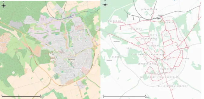
Veszprem is situated in the middle-western part of Hungary at 47°05’34” N and 17°54’49” E with the population of approximately 60,000 inhabitants. Hungary lies about halfway between the Equator and the North Pole, in the temperate zone, therefore, the weather is very changeable, mainly because it is influenced by the oceanic, continental, and the mediterranean climates. Thus, the annual average temperature in the city is approximately 10–12 °C (Central Transdanubia, 2017). Another important factors are the relief and the impact of the Carpathians, which is significant. The main contributors to air pollution in the city are public transport, private vehicles, public and domestic heating, and industrial activities (Fig. 1). Also, the impacts of the relief and the meteorological parameters are noticeable. Based on the air pollution index, the air quality in Veszprem is good (Air Quality Report, 2017).
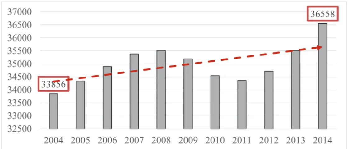
Based on the data of the Hungarian Central Statistical Office (2017), there has been a visible increase of the number of registered vehicles in the studied period (Fig. 2). All these vehicles moving on the streets result traffic congestion problems in Veszprem, especially during the morning (06:00–08:00) and evening (16:00–18:00) rush hours.
Fig. 1. Measurement area of the research project and its geographical location: (left) aerial view of the city (OpenStreetMap), (right) public transportation lines in the city (OpenStreetMap).
Fig. 2. Number or registered vehicles in the city of Veszprem between 2004 and 2014.
2.2. Meteorological data
For analyzing air quality, it is important to know the parameters that influence the ambient concentration of air pollutants. The selected relevant meteorological factors are the following: temperature (K); atmospheric pressure (hPa); wind speed (m/s), and precipitation (mm). The necessary meteorological data were supplied by the Institute of Radiochemistry and Radioecology of the University of Pannonia. The data were collected between 2004 and 2014. Their statistically processed version is shown in Fig. 3.
Fig. 3. Annual average values of meteorological parameters: (a) wind speed, (b) temperature, (c) atmospheric pressure, (d) precipitation.
33856
36558
32500 33000 33500 34000 34500 35000 35500 36000 36500 37000
2004 2005 2006 2007 2008 2009 2010 2011 2012 2013 2014
0 5 10 15 20
Wind speed [m/s]
280 282 284 286 288
Temperature [K]
1012 1014 1016 1018 1020
Atmospheric pressure [hPa]
0 50 100 150
Precipitation [mm]
2.3. Collection of ambient air quality data
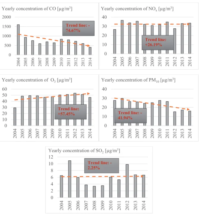
The different air pollutants concentrations (CO, NOx, O3, PM10, and SO2) were obtained from the automatic monitoring network system of the Hungarian Air Quality Network (OLM). Data observed between 2004 and 2014 were used in this study. Statistically processed data are shown in the following figures (Fig. 4).
Fig. 4. Yearly average concentration of the measured air pollutants: (a) carbon-monoxide, (b) nitrogen-oxides, (c) ozone, (d) particulate matter, (e) sulphur-dioxide.
0 500 1000 1500 2000
2004 2005 2006 2007 2008 2009 2010 2011 2012 2013 2014
Yearly concentration of CO [µg/m3]
Trend line: - 74.67%
0 10 20 30 40
2004 2005 2006 2007 2008 2009 2010 2011 2012 2013 2014
Yearly concentration of NOx[µg/m3]
Trend line:
+26.19%
0 10 20 30 40 50 60
2004 2005 2006 2007 2008 2009 2010 2011 2012 2013 2014
Yearly concentration of O3[µg/m3]
Trend line:
+57.45%
0 10 20 30 40
2004 2005 2006 2007 2008 2009 2010 2011 2012 2013 2014
Yearly concentration of PM10[µg/m3]
Trend line: - 41.94%
0 2 4 6 8 10 12
2004 2005 2006 2007 2008 2009 2010 2011 2012 2013 2014
Yearly concentration of SO2[µg/m3] Trend line: - 2.25%
2.4. Regression analysis
To study the relationship between the variables, regression analysis was used according to Douglas et al. (2012), Darlington (2016), and Xin (2009).
Statistical calculations have been used to analyze the extent to which the individual parameters such as temperature, solar radiation, wind direction, velocity, or relative humidity may be influenced by the concentration of different pollutants. The statistical method used is the regression calculation, also known as the correlation test. The essence is that we are looking for a relationship with a mathematical function between a dependent variable (result variable) and one or more explanatory variables. IBM SPSS Statistics has been used for the regression analysis. The following software outputs were used:
summary tables, variance analysis tables, regression coefficients, and statistical test tables containing the results of the hypothesis test (F-test, sum of square deviations, degrees of freedom, T-test). According to the calculations, in each case p value was less than 0.0001, which means that the results are very significant.
3. Results
The interconnection between the meteorological parameters, such as wind speed, temperature, air pressure, and precipitation and the concentration of certain major air pollutants (CO, NOx, O3, PM10, and SO2) was examined by using linear regression analysis. By determining the linear correlation coefficient (R) – also called Pearson product moment correlation coefficient –, the strength and direction of a linear relationship between two variables were determined.
The range of R was between –1 to +1, as shown in Table 1. The coefficient is symmetric. The closer the value to the endpoint the stronger the linear correlation, like in the case of CO concentration and wind speed (0.841). A perfect positive fit is achieved at R=+1, and a perfect negative fit is achieved at R=–1. On the contrary, if the value of R is close to 0, no or weak linear correlation can be determined meaning that there is a random, nonlinear relationship between the two variables, like in the case of SO2 concentration and atmospheric pressure (0.011).
Table 1. Linear correlation coefficients of the selected parameters
R CO NOX O3 PM10 SO2
Wind speed 0.841 0.635 0.723 0.277 0.074
Temperature 0.102 0.243 0.192 0.058 0.462
Atmospheric pressure 0.250 0.394 0.154 0.128 0.011
Precipitation 0.870 0.213 0.042 0.100 0.145
All meteorological parameters 0.884 0.740 0.862 0.344 0.490
Another tool of assessing relationships between variables is the coefficient of determinations (R2) that gives the proportion of the variance of one variable being predictable from the other (Table 2). It is the ratio of the explained variation to the total variation. The coefficient of determination ranges from 0 to 1 and denotes the strength of the linear association between the selected variables. The value shows the ratio of the data that is the closest to the line of best fit. If R2=1, the regression line goes through every single element of the scatter plot meaning that it approximates all of the data points. The farther a point is away from the regression line, the less variable can be explained.
Table 2. The coefficient of determinations of the selected parameters
R2 CO NOX O3 PM10 SO2
Wind speed 0.7070 0.4027 0.5222 0.0766 0.0053
Temperature 0.0104 0.0589 0.0370 0.0034 0.2142
Atmospheric pressure 0.0623 0.1549 0.0238 0.0165 0.0000 Precipitation 0.0076 0.0452 0.0017 0.0099 0.0212 All meteorological parameters 0.7820 0.5470 0.7430 0.1180 0.2400
The analysis shows (Fig. 5) that in the examined period, the CO concentration is strongly affected by the wind speed. The determination coefficient is 0.707, which means that there is a strong relationship between those variables. Contrast with that, in case of other meteorological parameters, CO shows low values of R2. Considering the relation between all meteorological parameters and the CO level, there is a high value (R2=0.7820), therefore, the positive relation were demonstrated.
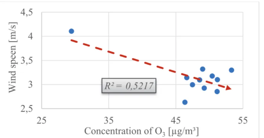
Furthermore, a moderate relation was observed in the case of the O3
concentration (Fig. 6). The coefficient of determinations was a bit lower (R2=0.5222), and the graph shows that between those two variables there is a negative linear correlation.
Fig. 5. Regression connection between the CO concentration and the wind speed.
Fig. 6. Regression connection between the O3 concentration and the wind speed.
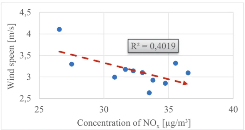
Similar tendency was observed between the concentration of NOx and the selected meteorological parameters (Fig. 7). The analysis confirmed a moderate relationship between the NOx concentration and the wind speed (R2=0.403). The relation of the NOx and all meteorological parameters could be stated also as moderate (R2=0.547).
R² = 0,7066
2,5 3 3,5 4 4,5
0 500 1000 1500 2000
Wind speen [m/s]
Concentration of CO [µg/m³]
R² = 0,5217 2,5
3 3,5 4 4,5
25 35 45 55
Wind speen [m/s]
Concentration of O3[µg/m³]
Fig. 7. Regression connection between the NOx concentration and the wind speed.
Relations between the PM10 concentration and the meteorological parameters were week. The highest values of R2 (Fig. 8) were noticed in the case of wind speed (R2= 0.0766). The analysis demonstrated a positive connection, however, the coefficient of determination with all meteorological parameters were low (R2= 0.1180).
Fig. 8. Regression connection between the PM10 concentration and the wind speed.
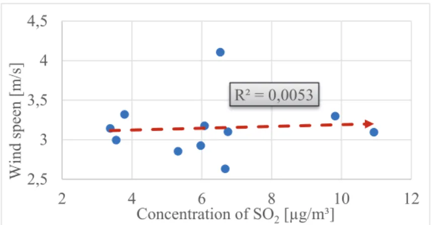
Similarly, to PM10 low connection was observed in the case of SO2 (Fig. 9).
The highest determination coefficient value (R2=0.2142) was between SO2 and temperature. The strength of the relation between SO2 and all meteorological
R² = 0,4019
2,5 3 3,5 4 4,5
25 30 35 40
Wind speen [m/s]
Concentration of NOx[µg/m³]
R² = 0,077
2,5 3 3,5 4 4,5
15 20 25 30 35
Wind speen [m/s]
Concentration of PM10[µg/m³]
Fig. 9. Regression connection between the SO2 concentration and the wind speed.
4. Discussion
In order to study the relationship between the CO, NOx, O3, PM10, and SO2
pollutants concentrations and the selected meteorological parameters, a linear regression analysis was carried out. The coefficient of the determinations (R2) between the CO, NOx, O3, PM10, and SO2 pollutants concentrations and the meteorological parameters comparing with other scientific researches are shown in Table 3.
Table 3. The coefficient of determinations of the selected parameters in this study and in other studies
R2 CO NOX O3 PM10 SO2
In this study 0.78 0.54 0.74 0.11 0.24
Sevda (2008) 0.48 0.28 0.75 * *
Barrero et al. (2006) * * 0.67 * *
Gupta et al. (2008) * 0.05–0.49 * 0.16–0.64 0.23–0.75
*not measured components
In accordance with the previous scientific works it can be stated, that the number of meteorological parameters included in regression equations were variable, and the analyses of the meteorological parameters affecting concentrations of air pollutants were diverse also. A strong dependence was obtained by Ocak (2008), who determined a 75% coefficient that means the 75%
of the O3 concentration depends on the wind speed, temperature, and relative humidity, which is close to the research results of Barrero et al., (2006) and also
R² = 0,0053
2,5 3 3,5 4 4,5
2 4 6 8 10 12
Wind speen [m/s]
Concentration of SO2[µg/m³]
to the results found in this study. Contrary to the research results of Ocak (2008), CO dependence was characterized by a strong relationship instead of a moderate one. In case of NOx, the results were ranged on a wide spectrum (0.05 – 0.54), but not any case was detected stronger than moderate. Gupta et al.
(2008) found the regression coefficients between PM10 and SO2 levels and meteorological factors as 0.16–0.75, which differs greatly from our findings, which may be due to the fact, that their measurements were carried out in three different areas (one residential site, one commercial site, and one industrial site).
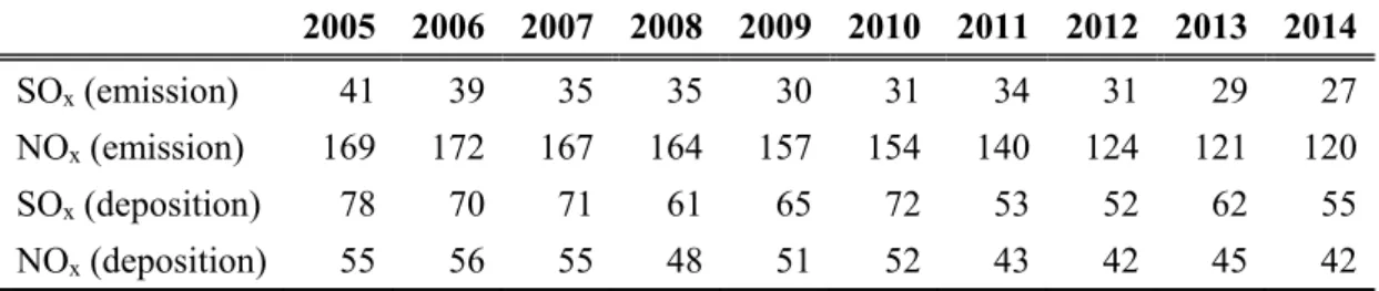
Besides the local emissions and meteorological conditions, the atmospheric long-range transport of pollutants influences the concentration field, too. For example, volcanic eruptions could have a significant effect on the SO2 and SO2−4
concentrations in air, as well as on the sulfur deposition. In 2014, a volcanic eruption started at the Barðarbunga fissure system in Iceland. There was little ash released in the eruption, but large amounts of SO2 were emitted into the atmosphere. For better understanding the pollution level in Veszprém county, the data sets were compiled from existing results of the atmospheric chemistry transport model ran by the European Monitoring and Evaluation Programme under the Convention on Long-range Transboundary Air Pollution (CEIP, 2016). The emissions and the estimated deposition of SOx and NOx in Hungary are shown in Table 4.
Table 4. Emission and estimated deposition of SOx and NOx in Hungary [unit: Gg(S);
Gg(N)]
2005 2006 2007 2008 2009 2010 2011 2012 2013 2014
SOx(emission) 41 39 35 35 30 31 34 31 29 27
NOx(emission) 169 172 167 164 157 154 140 124 121 120
SOx(deposition) 78 70 71 61 65 72 53 52 62 55
NOx(deposition) 55 56 55 48 51 52 43 42 45 42
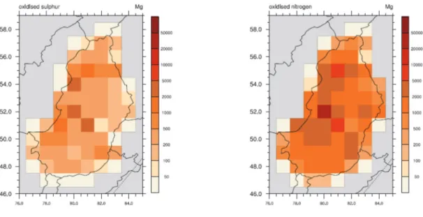
The spatial distribution and deposition from transboundary sources of SOx
and NOx are visible in Figs.10 and 11 (EMEP/MSC-W, 2014; Gauss et al., 2016). The amount of emitted contaminants has changed in proportion to the level of emissions. It can also be stated that the county was less exposed to SOx
depletion, while it was exposed to NOx pollution significantly.
Fig. 10. The spatial distribution of SOx and NOx (emissions).
Fig. 11. Deposition from transboundary sources of SOx and NOx (unit: mg(S)/m2, mg(N)/m2).
5. Conclusion
The aim of the present study was to determine the relationship between the CO, NOx, O3, PM10 and SO2 pollutants concentrations and selected meteorological parameters (wind speed, temperature, air pressure, and precipitation). It was not observed a significant change in the terms of the selected meteorological
parameters in Veszprem between 2004 and 2014. Variability of the values of wind speed, air pressure, and wind direction were not significant considering either the averages or the maximums or minimums. More extreme values were observed in the evolution of precipitation and temperature. In 2005, 2010, and 2014, the precipitation extremes were more significant than in the other years. It was noticeable, that among those years there were greatly drier years than the others, especially in 2011 and 2012. The temperature values were concerned too, and it has been found that there were a few outliers among the minimum and maximum values. The variability of averages was low. In the examined period, the highest and lowest values occured in the year of 2006. The concentration of air pollutants decreased between 2004 and 2014, except for concentration of nitrogen-dioxide and ozone. The main source of those air pollutants were transportation, which is determinative in Veszprem. The connection between the air pollutants and the meteorological parameters were demonstrated by regression analysis. The level of the relationship depends on the type of air pollutant and the meteorological parameter. The concentration of air pollutants were highly affected by the wind speed, since this parameter promotes the mixing and dilution of the pollutants. Among the analyzed parameters, CO and O3 indicate high determination values (>70%). In the case of the other pollutants, the low determination coefficient values could be explained by the low average annual emissions.
Acknowledgment: This study was supported by the Institute of Environmental Engineering and by the Institute of Radiochemistry and Radioecology of the University of Pannonia.
References
Air Quality Report, 2017: Air Quality Reports of the settlements based on the Hungarian Air Quality Monitoring Network. Hungarian Air Quality Monitoring Network – Reports Available:
http://www.levegominoseg.hu/reports (Accessed 13.01.2017)
Aynul, B., Warren, B. Kindzierski 2016: Evaluation of air quality indicators in Alberta, Canada – An international perspective. Environ. Int. . 92, 119–129
https://doi.org/10.1016/j.envint.2016.03.021
Barrero, M.A., Grimalt, J.O., and Canto, L., 2006: Prediction of daily ozone concentration maxima in the urban atmosphere. Chemometr. Intell. Lab. Sys. 80, 67–76
https://doi.org/10.1016/j.chemolab.2005.07.003
Casado LS, Shahrokh Rouhani, Carlos A. Cardelino, Adrian J. Ferrier, 1994: Geostatistical analysis and visualization of hourly ozone data, Atmos. Environ. . 28, . 2105–2118
https://doi.org/10.1016/1352-2310(94)90477-4 CEIP, 2016: Officially reported emission data
Országos Területfejlesztési és Területrendezési Információs Rendszer (TeIR) Available:
http://www.terport.hu/regiok/magyarorszag-regioi/kozep-dunantuli-regio (Accessed 13.01.2017) Casado, L.S., Rouhani, S., Cardelino, C.A., and Ferrier A.J. 1994: Geostatistical analysis and
visualization of hourly ozone data. Atmos. Environ. 28, 2105–2118.
https://doi.org/10.1016/1352-2310(94)90477-4
Chelani, A.B. and Rao, P.S. 2013: Temporal variations in surface air temperature anomaly in urban cities of India. Meteorol Atmos Phys 121, 215. https://doi.org/10.1007/s00703-013-0262-8
Chiu, K.H., Sree, U., Tseng, S.H., Wu, C-H., Lo, J-G., 2005: Differential optical absorption spectrometer measurement of NO2, SO2, O3, HCHO and aromatic volatile organics in ambient air of Kaohsiung Petroleum Refinery in Taiwan. Atmos. Environ. 39, 941–955.
https://doi.org/10.1016/j.atmosenv.2004.09.069
Cuhadaroglu, B. and Demirci, E. 1997: Influence of some meteorological factors on air pollution in Trabzon city. Energ. Build.25, 179–184. https://doi.org/10.1016/S0378-7788(96)00992-9
Darlington, R.D., 2016: Regression Analysis and Linear Models (Methodology in the Social Sciences). 1 Edition. The Guilford Press.
EMEP/MSC-W, 2014: EMEP MSC-W modelled air concentrations and depositions. Available:
http://www.emep.int/mscw/index.html (Accessed: 25.02.2019)
Gauss, M., Nyíri, A., Benedichtow, A., and Klein, H. 2016: Transboundary air pollution by main pollutants (S, N, O3) and PM – Hungary. MSC-W, ISSN:1890 - 0003
Gros, V., Sciare, J. and Yu, T., 2007: Air-quality measurements in megacities: Focus on gaseous organic and particulate pollutants and comparison between two contrasted cities, Paris and Beijing. Comp. Rendus Geosci. 339, 764-774. https://doi.org/10.1016/j.crte.2007.08.007
Gupta, A.K., Karar, K., Ayoob, S., and Kuruvilla, J., 2008: Spatio-temporal characteristics of gaseous and particulate pollutants in an urban region of Kolkata, India. Atmos. Res. 87, 103–115.
https://doi.org/10.1016/j.atmosres.2007.07.008
Hargreaves, P.R., Leidi, A., Grubb, H.J., Howe, M.T., and Mugglestone, M.A., 2000: Local and seasonal variations in atmospheric nitrogen dioxide levels at Rothamsted, UK, and relationships with meteorological conditions. Atmos. Environ. 34, 843–853.
https://doi.org/10.1016/S1352-2310(99)00360-X
Harinath, S. and Murthy, U.N., 2010: Spatial distribution mapping for air pollution in industrial areas – a case study, J. Industr. Poll. Cont. 26, 217–220.
Hiep, Duc, Shannon, I., Azzi, M., 2000: Spatial distribution characteristics of some air pollutants in Sydney. Math. Comput. Simulat. 54, 1–21.
https://doi.org/10.1016/S0378-4754(00)00165-8
Hungarian Central Statistic Office, 2017: Stock of Road transport. Available:
http://www.ksh.hu/transportt (Accessed 14.01.2017)
Li, L., Qian, J., Ou, C., Zhou, Y., Guo, C., and Guo, Y., 2014: Spatial and temporal analysis of Air Pollution Index and its timescale-dependent relationship with meteorological factors in Guangzhou. China. 2001–2011. Environ. Pollut. 190, 75–81.
https://doi.org/10.1016/j.envpol.2014.03.020
Luvsan, M.E., Shie, R.H., Purevdorj, T., Badach, L., Baldorj, B., and Chan, C.C. 2012: The influence of emission sources and meteorological conditions on SO2 pollution in Mongolia. Atmos.
Environ. 61, 542–549. https://doi.org/10.1016/j.atmosenv.2012.07.044
Mahapatra, P.S., Panda, S., Walvekar, P.P., Kumar, R., Das, T., and Gurjar, B.R., 2014: Seasonal trends. meteorological impacts. and associated health risks with atmospheric concentrations of gaseous pollutants at an Indian coastal city. Environ. Sci. Pollut. Res. 21, 11418–11432.
https://doi.org/10.1007/s11356-014-3078-2
Masiol, M., Hopke, P.K., Felton, H.D., Frank, B.P., Rattigan, O.V., Wurth, M.J., and LaDuke, G.H., 2017: Analysis of major air pollutants and submicron particles in New York City and Long Island. Atmos. Environ. 148, 203–214. https://doi.org/10.1016/j.atmosenv.2016.10.043
Minarro, M.D., Ferradas, E.G., Martinez, F.J.M., 2013: Influence of temperature changes on ambient air NO(x) chemiluminescence measurements. Environ. Monit. assess. 184, 5669–5678.
https://doi.org/10.1007/s10661-011-2372-4
Montgomery, D.C., Peck, E.A., and Vining, G., 2012: Introduction to Linear Regression Analysis. John Wiley & Sons.
Ocak, S. and Turailoglu, F.S. 2008: Effect of Meteorology on the Atmospheric Concentrations of Traffic-Related Pollutants in Erzurum, Turkey. J. Int. Environ. Appl. Sci. 3, 325–335.
Plaisance, H., Piechocki-Minguy, A., Garcia-Fougue, S., and Gallo, J.C., 2004: Influence of meteorological factors on the NO2 measurements by passive diffusion tube. Atmos. Environ.
38., 573–580. https://doi.org/10.1016/j.atmosenv.2003.09.073
Rodríguez, R., Casas, M.C., and Redaño, A., 2013: Multifractal analysis of the rainfall time distribution on the metropolitan area of Barcelona (Spain). Meteorol. Atmos. Phys. 121, 181.
https://doi.org/10.1007/s00703-013-0256-6
Wapler, K., 2013: High-resolution climatology of lightning characteristics within Central Europe.
Meteorol. Atmos. Phys. 122, 175. https://doi.org/10.1007/s00703-013-0285-1
Xin, Y., 2009: Linear Regression Analysis: Theory and Computing. 1 Edition. World Scientific Publishing Company.
Xu, J. and Zhu, Y., 1994: Some characteristics of ozone concentrations and their relations with meteorological factors in Shangai. Atmos. Environ. 28, 3387–3392.
https://doi.org/10.1016/1352-2310(94)00154-D