DOI:10.28974/idojaras.2020.3.3
IDŐJÁRÁS
Quarterly Journal of the Hungarian Meteorological Service Vol. 124, No. 3, July – September, 2020, pp. 349–361
Dependent weighted bootstrap for European temperature data: is global warming speeding up?
Csilla Hajas 1 and András Zempléni 2,*
1 Eötvös Loránd University Faculty of Informatics Department of Information Systems
Pázmány Péter sétány 1/C, H-1117 Budapest, Hungary
2 Eötvös Loránd University
Faculty of Science, Department of Probability Theory and Statistics Pázmány Péter sétány 1/C, H-1117 Budapest, Hungary
*Corresponding author E-mail: zempleni@caesar.elte.hu (Manuscript received in final form October 23, 2019)
Abstract⎯ Temperature changes are in the focus of climate research. There are many analyses available, but they rarely apply rigorous mathematics for assessing the results.
The main approach of this paper is the dependent weighted bootstrap. It is a simulation method, where both the fitted regression and the dependency among the data are taken into account. We present a simulation study showing that for serially dependent data it is the most accurate in case of estimating the coefficient in a linear regression.
This paper shows an analysis of the gridded European temperature data. We have used the 0.5°×0.5° grid of daily temperatures for 68 years (from 1950 to 2017), created by the European Climate Assessment. We investigated the speed of the global warming by changing the starting point of the linear regression. The significance of the differences between the coefficients was tested by the dependent weighted bootstrap. We have shown that the acceleration was significant for large regions of Europe, especially the central, northern and western parts.
The vast amount of results is summarized by a Gaussian model-based clustering, which is the suitable approach if we intend to have clusters that are spatially compact. The number of clusters was chosen as 13, by a suitably modified "elbow rule". This approach allows to compare the speed and acceleration of warming for different regions. The quickest warming in the last 40 years was observed in Central and Southwestern Europe, but the acceleration is more pronounced in Central Europe.
Key-words: dependent weighted bootstrap, global warming, linear models, model-based clustering
1. Introduction
Determining the speed of global warming is a very important and actual question, especially if significance of estimators is also tested. As mathematicians, we cannot give exact explanations for the changes, but we may try to reveal them and to estimate the statistical error of the estimates. This estimation is not easy at all, as in the data set there are various types of dependencies, which make the use of standard statistical techniques difficult.
Our main aim is to find those mathematical methods, which are most suitable for checking the significance of our results. There are numerous works in the area (see, e.g., Lu et al., 2005), where possible changepoints are introduced to capture the nonlinearity of monthly U.S. temperature data. We are convinced that using daily observations is worth for the efforts, as they convey much more information than, e.g., monthly or annual data.
Our approach is to capture the temporal changes by regression models, and then the spatial aspects can be taken into account by clustering. There are, of course, other approaches in the literature, where the spatial aspects are taken into consideration first (see, e.g., Jun et al., 2008), but our focus of attention is in the significance investigations for the univariate time series with complex and unknown dependence structure. For similar but monthly time series, Lund et al.
(1995) investigated the so-called periodic correlation structure. Their approach results in general 3p parameters, where p is the period. In our case p = 365, thus the number of parameters would be uncontrollable - considering that all are to be estimated for every grid point. Our model has about 60 parameters for the observation sites, which seems to be a good compromise.
The mathematical model in our case is the linear regression - not only for the whole, standardized data set, but for altogether 30 shorter data sets, which were got by omitting the first years sequentially, i.e., the kth set consists of the years (1950 + k, . . . , 2017). The main motivation behind this approach is that the actual changes are not easily captured by the commonly used functions (e.g., quadratic models cannot cope well with the complex structure of this data). Using this method we can detect if there is a change in the speed of the warming. For assessing the reliability of the results, we investigate different bootstrap approaches. We have to take care on the dependence in the data - the traditional solution to this phenomenon is the block bootstrap, covered in the book of Lahiri (2003). However, for the case of regression models, a new weighted bootstrap method has been developed by Wu (1986). A more recent approach by Shao (2010) is suitable for the case of dependent residuals - this is the one we used for assessing the reliability of the results and the significance of the change in speed of the temperature increase.
We are also interested in the spatial patterns of the processes. Thus, in Subsection 2.2 we apply a Gaussian model-based clustering (see, e.g., Fraley and Raftery, 2007) to the sequence of estimated coefficients.
We give details of the used models in Section 2. Section 3 is devoted to a simulation study on the bootstrap methods. Section 4 is about our results for the modeling of the temperature data. In Section 5 we formulate the conclusions.
2. Methods
In this section we briefly introduce the used methods. There is no need to introduce the linear models, as they are well-known to everyone. However, in order to assess the accuracy of the results we got by them, we needed special tools, as the data are both serially and spatially dependent. These will be explained in detail below.
2.1. Bootstrap
Bootstrap is a resampling method that can be used for assessing the properties of the estimators. There are many variants of the original idea of Efron (1979). One approach, designed especially for assessing the reliability of regression models is the weighted bootstrap of Wu (1986). However, all these standard methods are suitable only for the case of independent and identically distributed errors. In case of heteroscedasticity and/or dependency among the random error terms, the standard methods fail, as it is seen by our simulation study as well as in the classical paper of Singh (1981).
The dependent weighted bootstrap is suitable for these cases by choosing a resampling method that is capable of reproducing the dependence of the original observations. This is a relatively new concept, first introduced by Shao (2010). The traditional tool for such cases was the block bootstrap, which itself has several variants. There are available algorithms for choosing the block size, which minimize the standard error of the bootstrap estimators (Politis and White, 2004). However, it is reported in Shao (2010), that the new dependent weighted bootstrap has more favorable properties. We also check the methods in case of the linear regression, when we assume dependency among subsequent residuals. It turns out – as shown by our simulations – that the confidence intervals, based on the proposed weighted dependent bootstrap, have better coverage properties in the investigated cases.
In its original form (Wu, 1986), the weighted bootstrap sample was constructed from the estimated residuals of the regression model ri (i = 1, …, n, where n denotes the number of observations), by multiplying them with the weights wi, which were supposed to be i.i.d. (identically distributed), with E(wi) = 0 and Var(wi) = 1. These properties ensure that for the bootstrapped residuals wiri, we have E(wiri) = 0 and Var(wiri) = Var(ri). A natural choice may be the wi, for which P (wi = 1) = P (wi =
−1) = 0.5, thus practically choosing the same residuals as observed, but with random signs. There are of course other possible choices for the distribution of w (for details see Wu, 1986).
^
However, when the error terms are dependent, the simple method seen above does not work. The bootstrap data generating process must correspond to that of the observations. This can be achieved by the dependent weighted bootstrap, where the conditions E(wi) = 0 and Var(wi) = 1 still hold, but a dependence structure is assumed for the weights wi. In the original paper, Shao proposed a multivariate normal distribution, with covariance matrix
, = , (1)
where K is a kernel function and l is a suitable norming factor (bandwidth).
The generation of many dependent normal variates having such a covariance structure can be realized using the circular embedding algorithm of Dietrich et al.
(1997), which is implemented in the R package RandomFields.
The theoretical properties (consistency) of the dependent weighted bootstrap were proved originally by Shao under somewhat strong conditions (m-dependency of the weights), applicable, e.g., to the triangular kernel function. However, it has also been proved recently (Doukhan et al., 2015), that the method works for a simpler data generating process as well. Namely, the weights may come from an AR(1) series: = + (1 − ) , where εi is an i.i.d. sequence of normal distributions. The role of r is similar to that of l, they both determine the length of the memory in the sequence: a large r as well as a large l implies longer range dependence. Thus, the cases we investigate here have also favorable asymptotic properties.
One important problem is yet to be solved: how should we choose the parameter l? We have faced a similar question in the paper of Rakonczai et al.
(2014), where the block size of the bootstrap resampling had to be found. We determined it by the best fitting AR model (VAR in the bivariate case). The fit was measured by the variance of the estimator (or the trace of its covariance matrix in the bivariate case). To be more exact, in Rakonczai et al. (2014), the block size was determined as the , for which the estimated trace of the bootstrap covariance matrix was the nearest to the one derived from the fitted VAR model
= argmin
∈ ( ) − ∗ ∗ , ( 2 )
where ∗( ∗) = ∗( ∗|X ) (∗ refers to the bootstrap sample, i.e., the left hand side gives the covariance of the bootstrap sample based on block size b, under the observed sample X ). In this paper we have modified (2) on a way that the parameter was l from the kernel and to be able to estimate the variance of the mean, we fitted an AR(1) model to the data
= argmin ( ) − ∗ ∗ . ( 3 )
2.2. Clustering
Our data are spatio-temporal. Spatio-temporal data mining has been developed in the last few years (see for example Shekhar et al., 2011) or Chapter 10 in the book Giannotti and Pedreschi (2008). However, we prefer to use a simple, yet suitable and classical data mining tool, the clustering. The first idea for spatial clustering is to apply the density-based methods. However, it turned out that we have not got any valuable results by these methods. Thus, we rather applied the k-means clustering. This is a traditional, simple, and quick method even in our case of over 20000 data points in the 30 dimensional space. The method turned out to be suitable for detecting areas sharing similar properties, thus, also the spatial aspects were included in the analysis, especially when we used the model-based clustering. Here it is assumed, that the observations come from a multivariate normal distribution, with different parameters. The main question is if the covariances of the clusters are equal or different, and if different, what is the difference. Volume, shape, and orientation are the three aspects considered.
When applying the k-means clustering, it is a non-trivial question, how to determine the number of clusters. One may use the traditional elbow rule, based on the portion of the explained variance. The model-based clustering suggests a solution to this problem, as here an adapted version of the Bayesian information criterion (BIC) may be applied (see Fraley and Raftery, 2007). The method is implemented in the mclust package of R. BIC is traditionally defined here as the expression
= 2 log( ) − log( ),
where L denotes the value of the likelihood function at the optimum, n is the number of observations, and m the number of parameters in the model (B is
−1 times the "usual" BIC for regression model). So, in this approach the model with the largest BIC value is suggested to be chosen. However, in our case – most likely due to the vast amount of data – the BIC proposes a large number of clusters (around 100), so we came back to the old "elbow rule" and chose a clustering, after which the increase in the BIC is slowed down.
In our case, the results clearly proved that the model-based approach resulted in identifiable areas as clusters, which is very much preferred.
3. Simulations
First we checked the classical case, where the errors in the linear model are indeed independent and identically distributed. An independent sample with n = 100 from the model y = x + ε was simulated, with ε ∼ N (0; 1). The investigated methods were chosen so that the parameters are near to the ones used for the real data analysis:
1. the simple Efron-type bootstrap;
2. the weighted bootstrap for the residuals;
3. the dependent weighted bootstrap with AR(1) structure for the weights and normal innovations, as wn = 0.9wn−1 + √0.19ηn, where ηn is an i.i.d. standard normal;
4. the dependent weighted bootstrap with multivariate normal weights, the covariance was given by σi,j = 1 − | − |/ for l = 25.
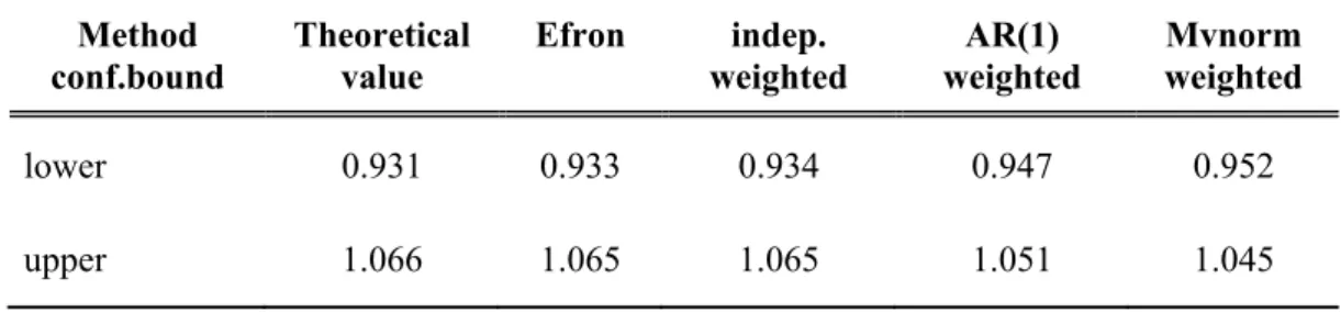
It can be seen from Table 1, that both the Efron-type and the independent weighted bootstrap give accurate results, while the intervals based on the two dependent weighted bootstrap methods are too narrow, which underlines that their application is unnecessary, if independence can be accepted. However, the difference is not too large.
Table 1. The effect of bootstrap type on the estimated confidence interval for the trend coefficient (now 1) in case of i.i.d. normally distributed error structure. For the dependent weighted bootstrap, the AR(1) coefficient was 0.9. The dependence for the multivariate normal weighted case was given by Eq.(1) with the triangular kernel. The number of repetitions was n = 500
Next we have simulated sequences of length n=23360 (the number of observations in our data set) with AR(1) structure for the residuals with r = 0.812 (the average of our estimators) and a trend coefficient of 8.6 ∗ 10−5 (again a typical value for our data set). The repetition size was 500, and we compared the performance of the three bootstrap methods, including the block-bootstrap with
Method conf.bound
Theoretical value
Efron indep.
weighted
AR(1) weighted
Mvnorm weighted
lower 0.931 0.933 0.934 0.947 0.952
upper 1.066 1.065 1.065 1.051 1.045
the optimal block size, based on the algorithm of Politis and White (2004). The results are shown in Table 2, containing 105-times the estimated values. Here we can observe the superiority of the weighted bootstrap, as it reproduces the theoretical quantiles the best – and the differences here are much more substantial than those of Table 1.
Table 2. 105 times the theoretical and estimated quantiles for the trend coefficient in case of normally distributed AR(1) error structure with r = 0.812 and a trend coefficient of 8.6 ∗ 10−5. The block bootstrap is too conservative with extreme quantiles; the independent weighted bootstrap on the other hand is too optimistic. The dependent weighted bootstrap (with the AR(1) dependence, determined by Eq. (3) turned out to be the best. The number of repetitions was 500.
method quantile 0.025 0.05 0.25 0.5 0.75 0.95 0.975 AR(1) process 6.64 6.95 8.05 8.53 9.12 10.11 10.43 block bootstrap 5.34 5.64 7.72 8.86 10.39 12.19 12.62 indep. weighted boot 7.62 7.75 8.30 8.61 8.94 9.41 9.50 dep. weighted boot 6.74 7.14 8.13 8.77 9.40 10.22 10.47
4. Applications
Temperature changes are in the focus of attention since global warming became a major threat to the ecosystem on Earth. There is a tremendous amount of information available on the subject (see, e.g., Weart, 2017 and the references therein), showing that the temperature sequences have started to rise from as early as 1960s. There are opinions about the link between NAO (North Atlantic Oscillation) index and low frequency variability of the climate (see, e.g., Cohen and Barlow, 2005). In our previous manuscript (Hajas and Zempléni, 2018) as a comparison, we have also investigated the residuals, after having removed the effect of the daily NAO index on the temperature time series. This effect was not substantial, but the use of these data allowed for checking the robustness of the results.
The used observations are 68 years of daily temperature data of the European Climate Assessment from 1950 to 2017 (E-OBS, http://www.ecad.eu). We have used the 0.5°×0.5° grid data, available for Europe and parts of Northern Africa.
This gridded database can be considered as a standard for climate analysis (see
Haylock et al., 2008). Its quality has been evaluated in Hofstra et al. (2009), and the results show that it may be considered reliable for most of Europe. However, especially in the African and Near Eastern region, there are missing periods of various length, which have to be taken into account. An earlier version of the same temperature data set was used in Varga and Zempléni, (2017), where the changes in the bivariate dependence structure were analyzed.
We have not investigated the time series in detail, but it is obvious that seasonality is its most important feature. So first we have standardized the data for every day of the year by simple nonparametric polynomial (Loess) smoothing, using both first- and second-order standardization for each grid point separately:
= ( − )/ , where T = 365 and 1 ≤ t ≤ 365 represents the day of the year. mt and st is the smoothed mean and standard deviation for day t, respectively.
These standardized daily data were used as a basis for the simple linear regression: = ( + ) + . We are interested in the steepness of the regression line (measured by the estimated coefficient αˆ), as well as in the strength of the model (as shown by the coefficient R2). These parameters were calculated for the data we have got by omitting the first k years (k = 1, …, 30):
i.e., in the kth equation we consider data from year k + 1 till 68, so the last model corresponds to approximately the last 40 years. This approach is motivated by the fact that the time series exhibit many features like abrupt changes or temporal decrease (especially in the first half of the data set), that are not possible to be captured by a seemingly simple quadratic regression.
The maximum value of the estimated regression coefficients together with the time of their occurrence is shown for each grid point in Fig. 1. We see that these maximal values occur for most of the cases at the very end of the investigated period. We have checked the reliability of the results for a grid of 10°×10° (the black rectangle on the right hand panel of Fig. 1) (using the weighted dependent bootstrap), and it turned out that for over 66% the grid points, at least 95% of the simulations gave at least k = 27 as the time point of the maximum, showing that the high values of the right hand side of Fig. 1 have not just been resulted by chance.
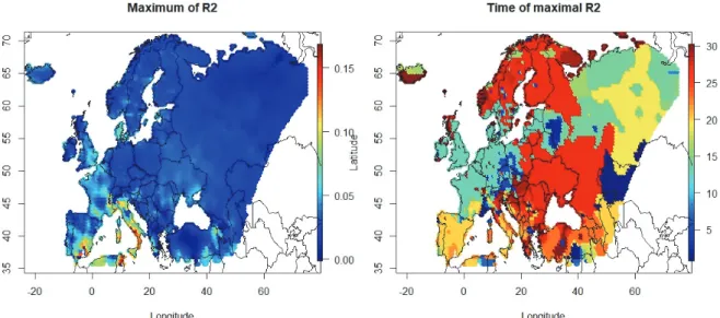
A similar plot for the strength of the model is Fig. 2. Not surprisingly, we see the larger values mostly in the regions with higher coefficients. The low values of R2 are quite natural, as there are many more nonlinear disturbances in the weather, compared to the relatively slow but steady global warming. It is interesting that for large areas of Western Europe we see an early occurrence, while the typical time points for Central and Northern Europe are again the late ones.
Fig. 1. Maximum of the regression coefficients for the grid points (left) and the time point of their occurrence (30 is the latest, right). On the right panel, a black rectangle shows the region, where the reliability of the results was checked.
Fig. 2. The maximal R2 value of the linear regression for the grid points (left) and the time point of their occurrence (30 is the latest, right).
One interesting question is the significance of the results for the climate data we have analyzed. We performed a small study, were the linear coefficient was defined as 10−4 and a simple AR(1) structure for the residuals was assumed
= 0.9 + √0.19 ,
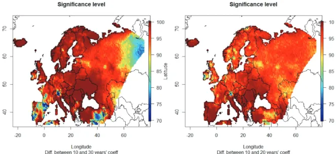
where the sequence ηn was i.i.d. standard normal. Here we have also used the dependent weighted bootstrap method introduced in Subsection 2.1, and we focused on the steepness coefficient of the linear model. It turned out that the estimators like this are not significant for much shorter series, but n ≥ 30∗365 is sufficient for α = 0.05%. We have pursued this idea further by applying the dependent weighted bootstrap method to our data with r = 0.9, which was chosen as an average solution of Eq. (3). Having repeated the simulations 100 times for each data point for k = 10, k = 20, and k = 30, we have got 3 times 100 coefficients for the grid points (let us denote them by x10, x20, and x30), respectively. We may estimate the significance of the increase of the coefficients by calculating the percentage of the pairs where x30 is larger than, e.g., x10. Such values are plotted on Fig. 3. We can see that the speeding up is highly significant for Scandinavia and large parts of Central Europe.
Fig. 3. Significance of the increase of warming, when the last 37 years (k = 30) are compared to the last 57 years (k = 10, left panel) and when the last 47 years (k = 20) are compared to the last 57 years (k = 10, right panel).
We have performed a model-based k-means clustering of the grid points for the regression coefficients. Similar approach was used for a completely different data in Hajas and Zempléni (2017). The clearly preferred model was the so-called VVV (ellipsoidal covariance structure with variable volume, shape, and orientation).
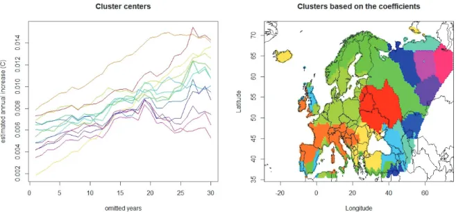
Fig. 4 shows the time-development of the 13 cluster centers as well as the clustering itself. Every single value is positive, in accordance with the widely accepted phenomenon of the global warming. This phenomenon was investigated at European level (e.g., in van der Schrier et al., 2013), proving the existence of the warming, at least from about 1980. But we can show much more: the most affected areas can also be identified. Almost all of the curves show a clear upward trend, i.e., in almost all cases the coefficient increases as the number of omitted years from the beginning of the investigated period increases. This means an acceleration of the temperature increase in the last part of the investigated period.
However, the changes in the coefficients (i.e., the speeding up of the temperature increase) are different in the clusters.
Fig. 4. Cluster centers (left) and the clustering (right), based on the regression coefficients for the grid points (13 clusters, based on the Gaussian mixture method).
The clusters differ mainly in their baseline level, the lines were otherwise quite parallel, at least up to k = 20, where an interesting change can be observed:
in some regions the annual increase remains nearly constant, while for others the speeding up continues. It is of definite meteorological interest to investigate which areas belong to the individual clusters. We may state that Central Europe belongs to the clusters with the highest acceleration of the temperature increase. Also a quick estimated increase is observed in the western part of the Mediterranean region and on Iceland, while the European part of Russia showed the slowest increase. It is, however, interesting that for the Iberian Peninsula the temperature increase is quick, but it has not increased further in the last period – in accordance
to Fig. 1, which shows that in this region the maximal coefficient occurs earlier than for most part of Europe (see the orange curve on the left panel of Fig. 4).
Similar pattern is observable for the northeast, where the increase is the slowest (see Figs. 1 and 3).
The quick, further temperature increase in the already warm regions might be interesting from a medical point of view as well, since the further warming of this region might result in quicker than expected outbreaks of tropical epidemics like malaria.
5. Conclusions
As a conclusion, we can claim that to analyze the temperature data by focusing on the last decades was a sound idea, as we found interesting patterns in the gridded temperature data. The Gaussian model-based clustering has resulted in a clear pattern of different regions, which might be a useful start for further climatic research.
The bootstrap is indeed an important tool in evaluating the significance of our results. However, one has to be aware of its properties. In case of dependent data, we have to take this dependence into account, when planning the bootstrap data generating process. We have compared the available methods and it turned out that the dependent weighted bootstrap is the most accurate in our case, where the dependency is simply modeled by an AR(1) process. The reason, that it outperforms the well-known block-bootstrap methods, might be the fact that here regression models were investigated.
Acknowledgement: We acknowledge the E-OBS dataset from the EU-FP6 project ENSEMBLES (http://ensembles-eu.metoffice.com) and the data providers in the ECA&D project (http://www.ecad.eu).
The research of A. Zempléni was supported by the Hungarian National Science Foundation (OTKA, K-81403).
References
Cohen, J. and Barlow, M., 2005: The NAO, the AO and Global Warming: How Closely Related? J.
Climte 18, 4498–4513. https://doi.org/10.1175/JCLI3530.1
Dietrich, C. R., Garry N. and Newsam, G.N., 1997: Fast and Exact Simulation of Stationary Gaussian Processes through Circulant Embedding of the Covariance Matrix, SIAM J. Scientific Comput. 18, 1088–1107. https://doi.org/10.1137/S1064827592240555
Doukhan, P., Lang, G., Leucht, A., and Neumann, M.H., 2015: Dependent wild bootstrap for the empirical process. J. Time Series Anal. 36, 290–314. https://doi.org/10.1111/jtsa.12106
Efron, B., 1979: Bootstrap methods: another look at the jackknife. Ann. Statistics 7, 1–26.
https://doi.org/10.1214/aos/1176344552
Fraley, C. and Raftery, E.A., 2007: Bayesian regularization for normal mixture estimation and model- based clustering. J. Classific. 24, 155–181. https://doi.org/10.1007/s00357-007-0004-5
Giannotti, F. and Pedreschi, D. (eds), 2008: Mobility, Data Mining and Privacy, Springer Verlag.
https://doi.org/10.1007/978-3-540-75177-9
Haylock, M., Hofstra, N., Klein T., Albert M. G., Klok, E.J., Jones, P.D., and New, M., 2008: A European daily high-resolution gridded data set of surface temperature and precipitation for 1950-2006. J.
Geophys. Res.: Atmospheres 113. https://doi.org/10.1029/2008JD010201
Hajas, C. and Zempléni, A., 2017: Chess and bridge: clustering the countries, Annales Univ. Sci.
Budapest., Sect. Comp. 46, 67–79.
Hajas, C. and Zempléni, A., 2018: Mathematical modelling European temperature data: spatial differences in global warming [Cited 2018 Oct 30]. Available from: https://arxiv.org/
abs/1810.13014
Hofstra, N., Haylock, M., New, M., and Jones, P.D., 2012: Testing E-OBS European high-resolution gridded data set of daily precipitation and surface temperature, J. Geophys. Res. Atmospheres 114.
https://doi.org/10.1029/2009JD011799
Jun, M., Knutti, R., and Nychka, D. W., 2008: Spatial analysis to quantify numerical model bias and dependence: how many climate models are there? J. Amer. Stat. Assoc. 103, 934–947.
https://doi.org/10.1198/016214507000001265
Lahiri, S.N., 2003: Resampling Methods for Dependent Data. Springer Verlag.
https://doi.org/10.1007/978-1-4757-3803-2
Lu, Q., Lund, R.B., and Seymour,P.L., 2005: An Update of United States Temperature Trends, J. Climate, 18, 4906–4914. https://doi.org/10.1175/JCLI3557.1
Lund, R.B., Hurd, H., Bloomfield, P., and Smith, R.L., 1995: Climatological Time Series with Periodic Correlation. J. Climate 11, 2787–2809.
https://doi.org/10.1175/1520-0442(1995)008<2787:CTSWPC>2.0.CO;2
Politis, D.N. and White, H., 2004: Automatic block-length selection for the dependent bootstrap, Econometric Rev. 23, 53–70. https://doi.org/10.1081/ETC-120028836
Rakonczai, P., Varga, L. and Zempléni, A., 2014: Copula fitting to autocorrelated data with applications to wind speed modelling, Annales Univ. Sci. R. Eötvös, Sect. Comp., 43, 3–19.
van der Schrier, G., van den Besselaar, E.J.M, Klein Tank, A.M.G. and Verver, G. , 2013: Monitoring European average temperature based on the E-OBS gridded data set, J. Geophys. Res.:
Atmospheres 118, 5120–5135. https://doi.org/10.1002/jgrd.50444 Shao, X., 2010: The dependent wild bootstrap, JASA, 105, 218–235.
https://doi.org/10.1198/jasa.2009.tm08744
Shekhar, S., Evans, M.R., Kang, J.M., and Mohan, P., 2011: Identifying patterns in spatial information: a survey of methods. Wiley Interdisc. Rev.: Data Mining Know. Disc. 1, 193–214.
https://doi.org/10.1002/widm.25
Singh, K., 1981: On the asymptotic accuracy of Efron’s bootstrap, Ann. Stat, 9, 1187–1194.
https://doi.org/10.1214/aos/1176345636
Varga, L. and Zempléni, A., 2017: Generalised block bootstrap and its use in meteorology, Adv. Stat. lim.
Meteorol. Oceanogr. 3, 55–66. https://doi.org/10.5194/ascmo-3-55-2017
Weart, S., 2017: The Discovery of Global Warming, [Cited 2019 Feb]. Available from https://history.aip.org/climate/ 20ctrend.htm#L_M066
Wu, C. F. J., 1986: Jackknife, Bootstrap and Other Resampling Methods in Regression Analysis (with discussion). Ann. Stat. 14, 1261–1350. https://doi.org/10.1214/aos/1176350142