DOI:10.28974/idojaras.2019.2.3
IDŐJÁRÁS
Quarterly Journal of the Hungarian Meteorological Service Vol. 123, No. 2, April – June, 2019, pp. 165–181
Weather model fine-tuning with software container-based simulation platform
Róbert Lovas1, Péter Kardos2, András Zénó Gyöngyösi*3, and Zsolt Bottyán4
1Institute for Computer Science and Control, Hungarian Academy of Sciences H-1132 Budapest, Victor Hugo u. 18-22., Hungary
2HungaroControl, Hungarian Air Navigation Services Pte. Ltd. Co.
H-1185 Budapest, Igló u. 33-35., Hungary
3Department of Climatology and Landscape Ecology, University of Szeged H-6722 Szeged, Egyetem u. 2., Hungary
4Institute of Military Aviation, National University of Public Service H-1083 Budapest, Ludovika ter 2., Hungary
*Corresponding Author E-mail: zeno@nimbus.elte.hu (Manuscript received in final form October 26, 2018)
Abstract⎯ Fine-tuning of a weather model requires immense computational resources, however, such capacities are usually available on non-homogeneous IT platforms. In addition, development and operational application are typically performed on different, heterogeneous systems (from laptops to dedicated HPC servers or cloud computing environments). To manage scalability and platform independent portability, a new layer – supporting state-of-the-art software container technology and batch processing – has been introduced. Encouraged by prior successful benchmark tests of the WRF model, the effect of model setup has been investigated over 10 different cases, tested on 30 different configurations. Including different parameterizations, the results of 300 different runs can be compared in a uniform database, yielding a sufficiently wide pool of samples in order to obtain the configuration of the modeling system optimal to the scope of our research, based on a relatively objective selection method. Continuously expanding database of near real-time preliminary outputs gives the opportunity for run-time steering of the experiments. This research currently benefits the development of an aviation meteorological support system, in the meanwhile, our contributions could be applied in an even wider aspect, either from the applicability of big data technology point of view, or with respect to the given best practice model setup.
Key-words: aviation meteorology, WRF model parameter optimization, docker software container technology, high performance computing, cloud computing
1. Introduction
All research that includes any kind of numerical weather modeling generally faced the nuisance of its immense computational requirement (see Section 2). This paper addresses the question whether there is a comfortable way to manage this computational background with significantly less manual effort instead of deep mining to benchmarking of various HPC (high performance computing) platforms, meanwhile the researchers can focus on their real expertise of meteorological details.
On the other hand, there is a fundamental change in the approach on HPC platform point of view. Many applications of such computing resources now based on cloud computing (Mell and Grance, 2011) environments that provide flexible and affordable solutions. Moreover, we are the witnesses of spreading of lightweight software container-based technologies (see Sections 3.1. and 3.2.).
Such technologies enable easy portability, encapsulation, and management of complex software stacks and long-running simulation scenarios, such as fine- tuning of numerical weather modeling. The first part of the paper covers the meteorological modeling background and findings, followed by the description of the applied virtualized and container-based software and hardware platform in details (see Section 3.3.).
Meanwhile, there is a new challenge for meteorologist community, as there is a worldwide soaring of unmanned aerial systems (UAS) which includes various types of unmanned aerial vehicles (UAV) from the bee-sized to 10 meters wingspan drones, their ground based controllers, and finally, the two-way air-to- ground communication infrastructure as well. These systems need various meteorological information about several atmospheric features depending on specific operational threshold of the specific aerial vehicles (e.g., wind speed, humidity), or the details of their missions (e.g., visibility, cloud cover, sun radiation, etc.).
In the framework of the recent research activity, a meteorological support system has been developed for UAS operations (Bottyán et al., 2013, 2014, 2015, 2017; Tuba et al., 2013; Bottyán, 2017; Tuba and Bottyán, 2018). The information is represented in such a manner that the users (including UAV operators, decision makers, etc.) may interpret (or decode) them correctly and easily, such as diagrams, charts, and reports in common coded formats. Information is delivered to the user in a fast, convenient, and accessible way that does not require experience in the use of any special software or hardware. Products are published on the public domain of the computing server itself, through web applications.
Outputs can be accessed by any web browser, with even hand-held mobile devices, or even on remote sites with low band data link coverage. Besides actual predictions, the server also provides archive NWP and observed data at each location (if available) for comparison by analogy purposes.
The weather engine of the system is the 3.9 version of the open source, community developed Weather Research and Forecasting (WRF) model (Skamarock et al., 2008), since it is flexibly scalable, proved to be usable for (even UAS) aviation meteorology purposes (Passner et al., 2009), and capable to assimilate UAS observed weather data (Passner et al., 2012; Jonassen et al., 2012; Reen and Dumais, 2018) besides other applications from its broad range of functionalities. WRF has multiple choices of parameter options. Planetary boundary layer schemes, that have significant effect on the flow structure and turbulence near the surface and in the lower troposphere, have 13, while surface layer sub-models have 8 different options, but each PBL option can handle only 2–4 different surface layer parameterization, which limits the number of possible combinations. Microphysics parameterization for the treatment of the atmospheric water content that is crucial in cloud and precipitation formation and icing processes could be selected from 27 different choices. Cumulus convection parameterizations that represent deep (and shallow) convection including thunderstorm development have 14 different options. Land surface model for the representation of processes in the soil layer, which provides lower boundary condition for the atmospheric variables has 7 choices available. Both long- and shortwave radiation have 8 different schemes, respectively, to consider radiation, which is crucial in the surface energy balance that governs processes close to the ground. Total count of all possible combinations (excluding unstable or prohibited combinations) is on the order of several hundred thousands.
However, the applicability of each scheme is well documented in the literature, and there are recommendations of working example combinations for given geographic locations (e.g., “CONUS” or “tropical” physics suites at the beginning of the WRF ARW Version 3.9) because of the complex interactions of all the parameterizations applied in the model, the optimal combination for a given location, application (or even meteorological situation) may be chosen by trial and error.
Although the operational weather prediction models of the Hungarian Meteorological Service are the ALADIN (Horányi et al., 1996, 2006) and AROME (Seity et al., 2011) models, WRF has also been extensively used and tested in various research projects in Hungary. WRF has been used in a diurnal analysis of shallow convection driven PBL height over dry soil in the Carpathian Basin (Acs et al., 2014; Breuer et al., 2014), in a comparison of microphysical schemes for the simulation of precipitation formation in convective clouds (Sarkadi, et al, 2016), and in the evaluation of cloud seeding using a bin microphysics scheme (Geresdi et al., 2017).
In addition, several additional studies were carried out to simulate severe storm activity in Hungary with the use of the WRF model (e.g., Csirmaz, 2015), but model sensitivity to horizontal resolution has mostly been tested and – according to our best knowledge – the effect of the choice of different parameterization setups and their interactions specifically in the Carpathian Basin
were not investigated yet, such as it has been done for the Continental US, Middle- East and North Africa (e.g., Zittis et al., 2014), or for tropical regions (e.g., Pérez et al., 2014; Noble et al., 2014, 2017).
The actual parameter settings for our current (operational) setup has been obtained through an extensive testing and evaluation process using conventional HPC methods, i.e., model system has been run sequentially with different options, for different cases, and the scores of each run were evaluated afterwards in order to select the best setup (Gyöngyösi et al., 2013). This process took for months and used the operative modeling platform prior to public deployment of the system.
Operative application of the preliminary system is being run four times per day on the platform of the National University of Public Service, Institute of Military Aviation. In addition, the model system has been successfully set up and tested in our docker container-based virtual machine environment. This architecture provides additional computing resources for further calibration thereof.
2. Model setup and meteorological results 2.1. Applied model configurations
All tests were performed on the Version 3.9 of the WRF model. The initial and 3-hourly boundary conditions were preprocessed from 0.25 degree resolution GFS model outputs. The model domain and the applied high resolution nest have been tailored for the needs of an operative UAS meteorological support. Parent domain (d01) has 91×75 cells at 9 km horizontal resolution, centered at N47.1°
and E019.3°. Nested domain (d02) contains 196×136 cells at 3 km resolution, covering the territory inside the state border of Hungary. Vertical levels were explicitly set at 30 σ-levels, with σ1 = 0.999 resulting in a lowest model level height z1 = 4 meters AGL following the method suggested by Shin et al., (2012).
Time series output of only the d02 nested domain was evaluated against observation data. However, operational integrations are performed every 6 hours on a 96-hour lead time, test runs for evaluation were carried out for 36-hour lead time each, initialized at 12Z on the previous day of interest, and the first 12-hour output were dropped as spin-up.
To keep the number of possible model settings on a manageable level, we have focused on those parameters which have significant impact on results and are crucial for our present purpose. Therefore, microphysics (MP), planetary boundary layer physics (PBL), surface layer physics (SFC), and cumulus schemes (CU) were altered in an appropriate manner (see Table 1 for the definitions of control file “namelist” options for each parameterization settings). In all cases, the very well established and widely used Noah Land Surface Model and RRTMG short- and longwave radiation schemes have been used. 14 different quality microphysics schemes were compared from the old and rather simplified representation of cloud and precipitation formation (such as Kessler or WSM3) to
the newest development of cloud microphysics (e.g., Thompson or P3). In addition, 4 cumulus and 3 PBL schemes were tested concurrently. Only those combinations were applied which are well documented, and that resulted in stable model run and results. The option for tropospheric wind (TOPO) is only available for the Yonsei University’s PBL scheme, which has also been tested in the fine- tuning. Remaining settings (domain configurations, spatial resolution, static inputs, soil texture and landuse, preprocessing methods, initialization, etc.) were kept identical for all ensemble members. Note that we do not refer hereby to the documentation of each single parameterizations, however, they are all well described in the already referenced description of WRF (Skamarock et al., 2008), or the corresponding source reference that can be found there. Altogether 30 different setups (treated as 30 members of an ensemble integration – ENS) have been loaded into our CQueue (i.e., container queue, see Sections 3.1 and 3.2 for more details) system for processing (Table 2). Note that ENS member # 1 corresponds to the operational model setup, that has been taken from previous test results (Gyöngyösi et al., 2013).
Table 1. Microphysics (MP), Cumulus (CU) and Planetary Boundary Layer (PBL) schemes (and their respective namelist options) applied for model fine-tunning
MP # CU # PBL #
Kessler 1 Kain-Fritsch 1 YSU 1
WSM 3-class simple ice 3 BMJ 2 MYNN 2.5 level 5 WSM 5-class 4 Grell-Freitas 3 Bretheron-Park/UW 9 Eta (Ferrier) 5 New Grell (G3) 5
WSM 6-class graupel 6
Goddard GCE 7
New Thompson graupel 8
Milbrandt-Yau 2-mom 9
Morrison 2-mom 10
CAM V5.1 5-class 11
WRF 2-mom 5-class 14
NSSL 2-mom 17
NSSL Gilmore 21
P3 1-category 50
Table 2. Ensemble members definition
ENS 1 2 3 4 5 6 7 8 9 10 11 12 13 14 15
MP 4 3 3 3 3 1 4 1 5 6 7 8 9 10 11
SFC 1 1 1 5 1 1 1 1 1 1 1 1 1 1 1
PBL 1 1 1 5 9 1 1 1 1 1 1 1 1
CU 1 1 1 1 1 2 2 2 2 2 2 2 2 2 2
topo 2 0 2 0 0 0 2 2 0 0 0 0 0 0 0 ENS 16 17 18 19 20 21 22 23 24 25 26 27 28 29 30
MP 14 50 1 6 11 17 5 6 7 8 9 10 11 21 50
SFC 1 1 1 1 1 1 1 1 1 1 1 1 1 1 1
PBL 1 1 1 1 1 1 1 1 1 1 1 1 1 1 1
CU 2 2 3 3 3 3 5 5 5 5 5 5 5 5 5
topo 0 0 2 0 0 0 0 0 0 0 0 0 0 0 0
2.2. Evaluation method and results
For the sake of an efficient fine-tuning, various weather situations have been considered for simulation. Ten days with such weather that has adverse effect on aviation safety (e.g., freezing rain, snow, fog, low ceiling, and thunderstorm) were picked up from recent records. Dates and corresponding significant weather are summarized in Table 3. All cases refer to a period of 24 hours, exactly equal to a calendar day from 00:00Z to 24:00Z.
Table 3. Case study dates tested in parameterization fine-tuning
Description Date
Warm front with freezing rain, following a long, extremely cold period January 31, 2017 Severe freezing rain caused by a warm front February 1, 2017
Off-season snow in spring April 19, 2017
Freezing day with thunderstorms May 3, 2017
Fog, low ceiling, freezing rain before the arrival of a cold front January 17, 2018
Mild snowy day February 20, 2018
Cold day with snows February 28, 2018
Snow to freezing rain transition in the evening March 2, 2018
Off-season dense fog March 28, 2018
Early summer day with lifted nocturnal convection May 2, 2018
All ensemble members were run for all cases resulting in 300 jobs altogether that were pushed into our CQueue worker for processing. Time series output at the location of each surface synoptic weather station and airport (34 stations altogether) within d02 were re-sampled every 5 minutes, converted from native model output variables (as model coordinate wind components or water vapor mixing ratio) into observation variables (wind direction and speed, dew-point) and pushed through CQueue system into a database for further processing (see Fig. 5). Prior to the whole procedure, this database has been filled up with archive surface observation data as well, so model forecasts and observation data were comparable on the SQL database level. In addition, 3-hourly input weather data from the driver GFS model, interpolated to the location of synoptic stations were also filled into the database for comparison and background (reference) model error assessment purposes. Both GFS and WRF model data were compared against observations available in time and space for the following variables: 2- meter temperature (T2m), 2-meter dew point (Td2m), and 10-meter wind speed (ws10m). Although in most of the investigated cases, precipitation was a significant phenomenon, we have excluded this parameter from the verification formula, since there were lot of observations considered from stations without a reliable precipitation data, so the errors yielded by precipitation comparisons would significantly distort the evaluation. In addition, while T2m, Td2m, and ws10m
measurements were available on an hourly basis, precipitation data cycles were different, making uniform evaluation problematic.
The comparison method was kept simple but may be improved easily by changing the query evaluation formula and reprocessing the database in a real- time manner on the fly within a mean of several seconds of database processing time. The method used currently is based on the square WRF model error compared to the square GFS input error, yielding positive increment for improvement and negative for worsening WRF model performance compared to the input driver GFS skills. These increments were averaged over observations (h∈{3, 6, 9, 12, 15, 18, 21, 24} as GFS provided data for these time steps) on a given day (d∈[1..D]; D = 10) for all s stations (s∈[1..S]; S = 34) to yield one single (overall) Re(p) error score for a given e∈[1..E]; ES = 30 ensemble member (setup) for a given p∈{T2m, Td2m, ws10m} parameter as defined in the following equation:
= ⋅ ⋅ ∑ ∑ ∑ , , − , , − , , , −
, , , (1)
where F stands for GFS or WRF forecast data (as indicated in the superscript) and O stands for observations, respectively.
An overall error score has been introduced by simply summing up the parameter error scores yielding one single score for a given ensemble member for the overall comparison.
= ∑ , (2)
where Se is the overall error score.
Comparison of Se overall error scores are presented in Fig. 1 on a box-plot diagram, showing significant improvement in model skills for most of the ensemble members. The × crosses represent means (most of them are above zero, indicating positive added value of WRF downscaling), horizontal lines are medians (all of them are above zero, showing that in most of the cases, the WRF results are closer to observations than the interpolated GFS data), vertical intervals show the absolute spread of skill scores, while boxes represent the inter-quartile range (IQR) of the deviations. In some cases, high positive outliers (those data which hit IQR threshold by more than 1.5 x IQR are represented by individual dots) are indicating extraordinarily positive results, as for ensemble members #14, #17, #22, #26, and
#30, while both absolute and IQR spreads are small by positive means and medians.
It can be noted that current operational setup (ensemble member #1) yields mainly positive improvement compared to the simple interpolation of GFS fields, however, many other setups provide significantly better results in most cases. All WRF members yielded at least one result that performed poorer than GFS, and in most setups both absolute and IQR spreads are significant. Best results were yielded by ensemble members #15 and #20 (highest mean and median scores), while the best IQR and absolute ranges were yielded by ensemble members #17 and #30 (most reliable setups with low spreads).
Fig. 1. Overall error scores for each ensemble member means (crosses), medians (horizontal lines), absolute spreads (vertical line intervals), IQR ranges (boxes), and
> 1.5×IQR outliers (dots).
In order to analyze the source of the large spread in the overall scores, the squared error differences have been summed up for e ensemble members instead of d cases as formulated in Eq.(3), which yielded the Rd(p) error of the day parameter. The box-diagram of the error-of-the-day scores (in a similar manner to the overall error score box-plots, Fig. 2) shows high absolute and IQR spreads only for snow-to-freezing-rain-transition cases (January 1, 2017 and March 2, 2018), and relatively narrow positive results besides. The highest improvements compared to the GFS skills were yielded on April 19, 2017 (the “off-season-snow- in-spring” case). This indicates the possibility of the source of model errors to be sensitive to inverse lapse rate situations. In such cases, however, the assimilation of further (e.g., UAS-based) vertical profile measurements from the boundary layer with higher horizontal, vertical, and time resolution may significantly improve the forecast skills.
= ⋅ ⋅ ∑ ∑ ∑ , , − , , − , , , −
, , . (3)
Fig. 2. Same as Fig. 1 for errors of the day showing less spread and higher added value for most cases besides two snow-to-freezing-rain-transition days on January 31, 2017 and March 2, 2018.
By the evaluation of the above results it can be concluded, that the value added by the costly high-resolution downscaling of global model results highly depends on the case selected, rather than the parameterization settings chosen. So in order to find the optimal parameterization, one order of magnitude higher number of cases should be considered instead of increasing the number of setups. In addition, evaluation formula which takes into account integral parameters (i.e., CAPE, CIN, precipitable water, etc.) or non-dimensional quantities for the evaluation of profile data instead of solely surface data comparison should be considered for the sake of a model system that is reliable for aviation (say 3 dimensional) purposes.
Moreover, fine-tuning of model settings other than physical parameterizations (such as nesting, vertical resolution, data assimilation and dynamical options) may also be taken into account.
3. Applied container-based cloud computing platform 3.1. Docker containers for portability
Docker technology is the most rapidly spreading open-source software container platform (www.docker.com). It simplifies the software dependency handling, and ensures portability between different hardwares, platforms, operating systems, and architectures, while supporting secure and agile deployment of new features.
For the purposes of easy involvement of computing resources, the most important factor is portability, which simplifies the setting up of the environment on a wide variety of host machines in physical and cloud environments.
Fig. 3. Comparison of traditional operating system virtualization with Docker software container technology including Docker hub for publishing and storing images.
Docker images encapsulate environment settings and implement software dependencies (e.g., binaries and libraries) through inheriting other images. Fig. 3 presents a comparison between the traditional operating system virtualization and the Docker software container technology. Docker also provides a simple command line interface to manage, download (pull), and create new images by Docker engine, but further sophisticated tools are also available for complex, workflow-oriented, and orchestrated usage scenarios, such as the Occopus cloud and container orchestrator tool (Kovacs and Kacsuk, 2018).
A related work on performance measurement compares high performance computing resources in cloud and physical environment, with and without utilizing the Docker software container technology (Vránics et al., 2017). The results show that the performance loss caused by the utilization of Docker is 5–10%, which is negligible compared to the 10–15-fold improvement in deployment time. The comparison shows that the expected performance of cloud resources is slightly lower than the performance of physical systems.
3.2. CQueue container queue service
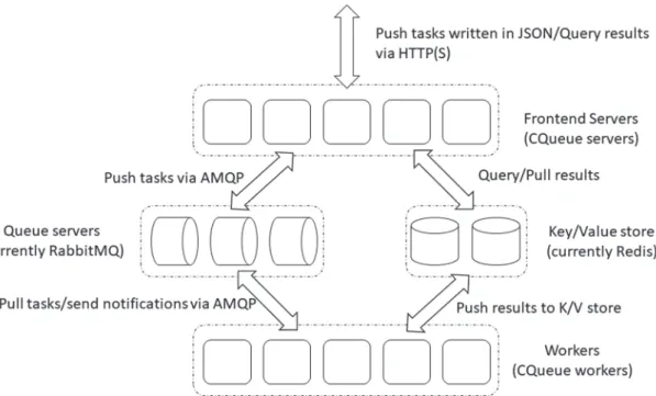
Since Docker does not provide pull model for tasks execution (its Swarm cluster approach uses push execution model), the new CQueue framework provides a lightweight queue service for processing tasks via application containers. The framework consist of four main components (see Fig. 4): (i) one or more CQueue server(s), which act(s) as frontend(s) and receive(s) the container based task requests; (ii) a queue server schedules the tasks requests for workers; (iii) CQueue workers that pull tasks from the queue server; and (iv) a key-value store that backups the state and the output of the finished tasks. Currently queuing is handled by RabbitMQ, and Redis is used as the key-value store. The frontend server and the worker components are written in golang and they have a shared code-base. All of the components are running inside Docker containers and can be scaled based on their utilization. The design goals of the framework is to use standard interfaces and components to create a generic job processing middleware.
The framework is built for executing Docker container, based tasks with their specific inputs. Environment variables and other input parameters can be specified for each container also. CQueue uses an unique ID to identify the pushed tasks, and the user has to specify it. The ID, the application container, and the inputs of the task must be specified in standard JSON (JavaScript Object Notation) format.
The CQueue server receives the tasks via a REST-Like API. After this step, the server transforms the JSON formatted tasks to standard AMQP (Advanced Message Queuing Protocol) messages and pushes them to the queue server. The workers pull the registered tasks from the queue server via the same AMQP protocol and execute them. One worker process one task at a time. After the task is completed, the workers send a notification to the queue server and this task will
be removed from the queue. The worker continuously updates the status (registered, running, finished, or failed) of the task with the task’s ID in the key- value store. When the task is finished or failed, the worker stores the stdout and stderr of task in the key-value store as well. The status of a task and the result can be queried from the key-value store through the CQueue server. The output of the task is not processed, it is stored in the key-value store in its original format.
Fig. 4. CQueue architecture.
3.3. Virtualized architecture at large
As Fig. 5 depicts, resources have been involved from two Hungarian large-scale research infrastructures, MTA Cloud (cloud.mta.hu) and Agrodat Cloud (agrodat.hu) in order to execute the container based WRF simulations.
MTA Cloud is a federated community cloud, jointly operated by the MTA Wigner Data Center (WDC) and the Institute for Computer Science and Control (MTA SZTAKI). The recently opened OpenStack (Wen et al., 2012) and Docker container-based cloud infrastructures combine resources from WDC and MTA SZTAKI relying on the nationwide academic Internet backbone and other federated services, e.g., eduGain for authentication and authorization. The total capacity of the two deployed sites is 1160 virtualized CPU with 3.3 TB memory and 564 TB storage facility.
Fig. 5. The major components and their interactions of the elaborated IT architecture.
On the other hand, during the numerical weather modeling, the Agrodat Cloud was used heavier, therefore, we introduce it with more details. The Agrodat Cloud is a more specialized IaaS cloud, its main aim to support agriculture related research based on OpenNebula 5.2 cloud middleware (Moreno-Vozmediano et al,, 2012). The underlying virtualization technique is KVM (hardware virtualization), and storage is provided both by a Ceph (Weil et al., 2006) distributed storage cluster and a QCOW2 store. Users can manage the cloud resources via browser based graphical interface (Sunstone) or via an EC2 interface. Additionally, an S3 based storage is part of the infrastructure (via RadosGW of Ceph). Currently 4 VM hosts (HPE ProLiant DL385p Gen8 and Dell PowerEdge R815 models) are allocated for the cluster with combined 144 CPU cores and 512GB RAM:
• Host 1: 2x AMD Opteron(tm) processor 6376 2.3GHz CPU (32 cores total), 128GB RAM,
• Host 2: 4x AMD Opteron(tm) processor 6262 HE 1.6GHz CPU (64 cores total), 256GB RAM,
• Host 3: 4x AMD Opteron(tm) processor 6164 HE 1.7GHz CPU (48 cores total), 128GB RAM.
Storage is available for the cluster as follows:
• 18.1TB QCOW2 storage,
• 31.5TB Ceph based distributed storage.
Networking is provided by Cisco Nexus 3548 (10Gb), and HP 5920 (10Gb Ethernet) switches. Ceph storage nodes are connected via 2x 10Gb Ethernet links to the network. Additionally, 1Gb Ethernet switches are used for management purposes.
On both clouds, the Docker container platform with CQueue (see Sections 3.1 and 3.2) enable the pull execution model for the fine-tuning of numerical weather modeling, i.e., each Cqueue worker on the launched virtual machines of the given cloud fetches the WRF jobs from the Meteor24 server one-by-one when worker becomes idle. It is also necessary to fetch the already prepared and published WRF container (see Vranics et al., 2017) from the public Docker Hub, but only once at the beginning of the simulation. The WRF jobs are prepared according to Section 2 using the data from the Global Forecasting System (GFS), and the progress and simulation results (stored in mySQL) can be accessed remotely. Total 300 jobs were added to CQueue system in our investigation. The average of 3 hour 38 minutes runtime of workers varies between 1 hour14 minutes to 11 hours 59 minutes depending on which parameterization scheme was applied in that specific setting. As 8–12 virtual machines provided computing capacity for CQueue workers in our experiment at the same time, the total processing period was less then 8 days. Of course, because of the scalability of the whole system, it can be decreased significantly with involving more virtual machines in an easy manner.
4. Related works and conclusion
Comparing to the traditional parallel (multi-threaded or message passing-based) execution of modeling, our approach takes benefits of the distributed computing paradigm as well, even in heterogeneous computing environments. In this way, we leverage on the parallel execution inside the given multi-core computing node, but theoretically, arbitrary number of different executions are allowed at the same time in a distributed manner, involving further available computing nodes (e.g., traditional servers, cluster nodes, or virtual machines in the cloud). This type of
loosely coupled and heterogeneous systems require special methods and tools to handle the complex distributed management and software stack portability issues.
There are several software container and (mostly cloud-based) automatic management tools addressing the above described problems, such as the widely used Kubernetes (Burns et al., 2016) and Tosca (Binz et al., 2014). Recently, new emerging tools are also appearing in this field, such as MiCADO (Kiss et al., 2017) and Occopus (Kovacs and Kacsuk, 2018), for distributed execution of simulations. The enlisted tools are more feature-rich products, but CQueue became a proven and promising approach leveraging on the presented WRF results and further application areas (see its use case for Industry 4.0 by Lovas et al., 2018) since it is similarly robust distributed computing technology but having significantly lower entry-barrier for non-IT specialist and not steep learning curve comparing to its competitors.
Concerning WRF related containerization works, there are also related works, (Hacker et al., 2017) but (among others) they did not provide such convenient but at the same time very robust approach like our CQueue container queue oriented solution. This tool provided valuable results for our research project, and proved that it is an efficient way to manage this kind of fine tuning.
As all results of finished jobs are available during the processing phase, we are able to add those new jobs into the schedule list which may serve promising additional information on the accuracy of various parameterization settings ensuring the effectiveness and time saving of the research project. Therefore, this tool is now ready to process plenty of jobs (magnitude of 1000) and to serve valuable information on appropriate parameterization settings for further research.
Acknowledgement: This work was supported by the European Regional Development Fund under Grant no. GINOP 2.3.2-15-2016-00007 (“Increasing and integrating the interdisciplinary scientific potential relating to aviation safety into the international research network at the National University of Public Service - VOLARE”). The project was realized through the assistance of the European Union, and co-financed by the European Regional Development Fund. On behalf of Project “Weather Research and Forecasting (WRF) - Benchmark & Orchestration” we thank for the usage of MTA Cloud that significantly helped us achieving the results published in this paper.
References
Ács, F., Gyöngyösi, A.Z., Breuer, H., Horváth, Á., Mona, T., and Rajkai, K., 2014: Sensitivity of WRF- simulated planetary boundary layer height to land cover and soil changes. Meteorol. Z. 23, 279–293.
Agrodat.hu project website. Accessed: 2018-06-17. https://doi.org/10.1127/0941-2948/2014/0544 Binz, T., Breitenbücher, U., Kopp, O., and Leymann, F., 2014: Tosca: Portable automated deployment
and management of cloud applications. In Advanced Web Services. 527–549. Springer.
Bottyán, Zs., Wantuch, F., Gyöngyösi, A.Z., Tuba, Z., Hadobács, K., Kardos, P., and Kurunczi. R., 2013:
Forecasting of hazardous weather phenomena in a complex meteorological support system for UAVs. World Acad. Sci. Engin. Technol. 7, 646–651.
Bottyán, Zs., Wantuch, F., and Gyöngyösi, A.Z., 2014: Forecasting of hazardous weather phenomena in
Bottyán, Zs., Gyöngyösi, A.Z., Wantuch, F., Tuba, Z., Kurunczi, R., Kardos, P., Istenes, Z., Weidinger, T., Hadobacs, K., Szabo, Z., Balczo, M., Varga, A., Birone Kircsi, A., and Horvath, Gy., 2015:
Measuring and modeling of hazardous weather phenomena to aviation using the Hungarian Unmanned Meteorological Aircraft System (HUMAS). Időjárás 119, 307–335.
Bottyán, Zs., 2017: On the theoretical questions of the uas-based airborne weather reconnaissance. In (Eds.: Bottyán, Zs., and Szilvássy, L.) Repüléstudományi Szemelvények: A közfeladatot ellátó repülések meteorológiai biztosításának kérdései. ISBN:978-615-5845-26-0, Nemzeti Közszolgálati Egyetem Katonai Repülő Intézet, Szolnok. 97–118.
Bottyán, Zs., Tuba, Z., and Gyöngyösi, A.Z., 2017: Weather forecasting system for the unmanned aircraft systems (uas) missions with the special regard to visibility prediction, in Hungary. In (Eds. Nádai L. and Padányi J.) Critical Infrastructure Protection Research: Results of the First Critical Infrastructure Protection Research Project in Hungary. Topics in Intelligent Engineering and Informatics; 12. ISBN:978-3-319-28090-5, 23–34. Springer International Publishing, Zürich.
Breuer, H., Ács, F., Horváth, Á., Németh, P., and Rajkai. K.: Diurnal course analysis of the WRF- simulated and observation-based planetary boundary layer height. Adv. Sci. Res. 11, 83–88.
(doi:10.5194/asr-11-83-2014)
Burns, B., Grant, B., Oppenheimer, D., Brewer, E., and Wilkes, J., 2016: Borg, omega, and kubernetes.
Commun. ACM, 59(5): 50–57. https://doi.org/10.1145/2890784
Csirmaz, K, 2015: A new hail size forecasting technique by using numerical modeling of hailstorms: A case study in Hungary. Időjárás 119,443–474.
Docker - Build, Ship, and Run Any App, Anywhere. https://www.docker.com, Accessed: 2017-10-30.
Geresdi I, Xue L, and Rasmussen R., 2017: Evaluation of orographic cloud seeding using a bin microphysics scheme: Two-dimensional approach. J App Met Clim. 56, 1443–1462.
https://doi.org/10.1175/JAMC-D-16-0045.1
Gyöngyösi, A.Z., Kardos, P., Kurunczi, R., and Bottyán, Zs., 2013: Development of a complex dynamical modeling system for the meteorological support of unmanned aerial operation in Hungary. In 2013 International Conference on Unmanned Aircraft Systems (ICUAS): Conference Proceedings,. 2013.05.28-2013.05.31. Atlanta (GA), ISBN: 978-1-4799-0815-8, 8–16, Atlanta, 2013. IEEE.
Hacker, J.P., Exby, J., Gill, D., Jimenez, I., Maltzahn, C., See, T., Mullendore, G., and Fossell, K., 2017:
A containerized mesoscale model and analysis toolkit to accelerate classroom learning, collaborative research, and uncertainty quantification. Bull. Amer. Meteorol. Soc., 98, 1129–1138.
https://doi.org/10.1175/BAMS-D-15-00255.1
Horányi A., Ihász I. and Radnóti G., 1996: ARPEGE/ALADIN: a numerical weather prediction model for Central-Europe with the participation of the Hungarian Meteorological Service. Időjárás 100, 277–301.
Horányi A., Kertész S., Kullmann L., and Radnóti G., 2006: The ARPEGE/ALADIN mesoscale numerical modeling system and its application at the Hungarian Meteorological Service. Időjárás 110, 203–227.
Jonassen, M.O., Olafsson, H., Agustsson, H., Rognvaldsson, O., and Reuder, J., 2012: Improving high- resolution numerical weather simulations by assimilating data from an unmanned aerial system.
Mon. Weather Rev. 140, 3734–3756. https://doi.org/10.1175/MWR-D-11-00344.1
Kiss, T., Kacsuk, P., Kovacs, J., Rakoczi, B.,Hajnal, A., Farkas, A., Gesmier, G., and Terstyanszky, G., 2017: Micado—microservice-based cloud application-level dynamic orchestrator. Future Generation Computer Systems. https://doi.org/10.1016/j.future.2017.09.050
Kovács, J., and Kacsuk, P., 2018: Occopus: a multi-cloud orchestrator to deploy and manage complex scientific infrastructures. J. Grid Comput. 16, 19–37. https://doi.org/10.1007/s10723-017-9421-3 Lovas, R., Farkas, A., Marosi, A.Cs., Acs, S., Kovacs, J., Szaloki, A., and Kadar, B., 2018: Orchestrated
platform for cyber-physical systems. Complexity 2018, Article ID 8281079, 16 pages, https://doi.org/10.1155/2018/8281079
Moreno-Vozmediano, R., Montero, R.S., and Llorente, I.M., 2012: Iaas cloud architecture: From virtualized datacenters to federated cloud infrastructures. Computer, 45, 65–72.
https://doi.org/10.1109/MC.2012.76
Mell, P. and Grance, T., 2011: The NIST definition of cloud computing. Technical Report SP 800-145, National Institute of Standards and Technology Gaithersburg, MD, United States.
MTA Cloud. https://cloud.mta.hu, Accessed: 2018-06-18.
Noble, E., Druyan, L.M. and Fulakeza, M., 2014: The sensitivity of WRF daily summertime simulations over West Africa to alternative parameterizations. Part I: African wave circulation. Mon. Weather Rev. 142, 1588–1608. https://doi.org/10.1175/MWR-D-13-00194.1
Noble, E., Druyan, L.M., and Fulakeza, M., 2017: The sensitivity of WRF daily summertime simulations over West Africa to alternative parameterizations. Part II: precipitation. Mon. Weather Rev. 145, 215–233. https://doi.org/10.1175/MWR-D-15-0294.1
Passner, J.E., Dumais jr., R.E., Flanigan, R., and Kirby, S., 2009: Using the Advanced Research version of the Weather Research and Forecast model in support of ScanEagle unmanned aircraft system test flights. ARL Technical Report ARL-TR-4746, Computational Information Sciences Directorate, U.S. Army Research Laboratory: White Sands Missile Range, NM.
Passner, J.E., Kirby, S., and Jameson, T., 2012: Using real-time weather data from an unmanned aircraft system to support the Advanced Research version of the Weather Research and Forecast model.
ARL Technical Report ARL-TR-5950, Computational Information Sciences Directorate, U.S.
Army Research Laboratory: White Sands Missile Range, NM.
Pérez, J.C., Díaz, J.P., González, A., Expósito, J., Rivera-López, F., and Taima, D., 2014: Evaluation of WRF parameterizations for dynamical downscaling in the Canary Islands. J. Climate, 27, 5611–
5631. https://doi.org/10.1175/JCLI-D-13-00458.1
Reen jr., R.E., and Dumais B.P., 2018: Assimilation of aircraft observations in highresolution mesoscale modeling. Adv. Meteorol. 2018. 1–16. https://doi.org/10.1155/2018/8912943
Sarkadi N., Geresdi I., and Gregory T., 2016: Numerical simulation of precipitation formation in the case orographically induced convective cloud: Comparison of the results of bin and bulk microphysical schemes. Atmos. Res. 180, 241-261. https://doi.org/10.1016/j.atmosres.2016.04.010
Seity Y., Brousseau P., Malardel S., Hello G., Bénard P., Bouttier F., Lac C., and Masson V., 2011: The AROME-France Convective-Scale Operational Model, Mon. Weather Rev. 139, 976–991.
https://doi.org/10.1175/2010MWR3425.1
Shin, H.H., Hong, S-Y., and Dudhia, J., 2012: Impacts of the lowest model level height on the performance of planetary boundary layer parameterizations. Mon. Weather Rev.140, 664–682.
https://doi.org/10.1175/MWR-D-11-00027.1
Skamarock, W.C., Klemp, J.B., Dudhia, J., Gill, D.O., Barker, D.M., Duda, M.G., Huang, X-Y., Wang, W., and Powers, J.G., 2008: A description of the Advanced Research WRF version 3.. NCAR Tech. Note NCAR/TN-475+STR, National Center of Atmospheric Research.
doi:10.5065/d68s4mvh
Tuba, Z., Vidnyánszky, Z., Bottyán, Zs., Wantuch, F., and Hadobács, K., 2013: Application of analytic hierarchy process in fuzzy logic-based meteorological support system of unmanned aerial vehicles. Acad. Appl. Res. Military Sci. 12, 221–228.
Tuba Z. and Bottyán, Zs., 2018: Fuzzy logic-based analogue forecasting and hybrid modeling of horizontal visibility. Meteorol. Atmos. Phys. 130, 265–277.
https://doi.org/10.1007/s00703-017-0513-1
Vránics, D.F., Lovas, R., Kardos, P., Bottyán, Zs., and Palik, M., 2017: WRF benchmark measurements and cost comparison. virtualized environment versus physical hardware. Repüléstudományi Közlemények, 29, 257–272.
Weil, S.A., Brandt, S.A., Miller, E.A., de Long, D., and Maltzahn, S., 2006: Ceph: A scalable, high- performance distributed file system. In Proceedings of the 7th symposium on Operating systems design and implementation. USENIX Association. 307–320.
Wen, X., Gu, G., Li, Q., Gao, Y., and Zhang, X., 2012: Comparison of open-source cloud management platforms: Openstack and opennebula. 2457–2461.
Zittis, G. Hadjinicolaou, P., and Lelieveld, J., 2014: Comparison of WRF Model Physics Parameterizations over the MENA-CORDEX Domain. Amer. J. Clim.Change 3, 490–511.
https://doi.org/10.4236/ajcc.2014.35042