IDŐJÁRÁS Quarterly Journal of the Hungarian Meteorological Service

DOI:10.28974/idojaras.2020.4.6

IDŐJÁRÁS

Quarterly Journal of the Hungarian Meteorological Service Vol. 124, No. 4, October – December, 2020, pp. 521–539

Estimation of Dew Point Temperature in Different Climates of Iran Using Support Vector Regression

Mohammad Nazeri-Tahroudi¹ and Yousef Ramezani^2,*

1 Department of Water Engineering, University of Birjand, Birjand, Iran

2 Department of Water Engineering, University of Birjand, Birjand, Iran

*Corresponding author E-mail: y.ramezani@birjand.ac.ir (Manuscript received in final form November 11, 2019)

Abstract The prediction of global climate change using the values recorded in a statistical period requires a precise method that can accurately identify the fluctuations of these changes. By patterning these changes, the parameter values for the years or future periods are predicted, or the statistical gap can be eliminated. In this research, meteorological data of six stations in different climates of Iran were used to model and estimate the values of the dew point temperature (DPT). The stations studied are Ahvaz, Urmia, Kerman, Gorgan, Rasht, and Babolsar. In order to estimate the DPT values, support vector regression was used, and to optimize the parameters of the support vector regression model, the ant colony algorithm was used. In this study, four different input patterns of meteorological data have been investigated as input of the support vector regression model. Pattern I with seven inputs (monthly minimum, maximum, and average air temperatures, monthly precipitation, saturation vapor pressure, actual vapor pressure and relative humidity), Pattern II with three inputs (monthly average air temperature, saturation vapor pressure, and actual vapor pressure), Pattern III with two inputs (monthly minimum and maximum air temperatures), and Pattern IV with an input (monthly average air temperature) were used. It is recommended that if the number of inputs in the model is small, the model will be more user-friendly. Based on the results of analyzing different patterns, it can be concluded, that Pattern III is the suitable pattern for estimating DPT values at the stations studied in different climates of Iran based on the three criteria of root mean square error (RMSE), Nash–Sutcliffe model efficiency coefficient (NSE), and coefficient of determination (R²). Overall, the results showed that the selected pattern increases the accuracy of the model by up to 24% compared to the conventional model.

Key-words: Ant Colony Algorithm, FAO Penman – Monteith, Modeling, Nonlinear Regression.

1. Introduction

Dew occurs when the temperature is equal to the dew point temperature (DPT).

These conditions occur on the ground for two important reasons. First, the propagation of longwave radiation makes the surface of the ground cool in the night. For condensation, temperature need to be reduced to DPT. Second, often the soil provides dew point moisture. That is, wet and warm soils can help to form dew. Cooling of wet soil during the night will cause condensation, especially in clear nights. Clear nights allow long wavelengths radiation have max propagation to space. The cloudy sky can absorb a portion of the longwave radiation and reflect the other part back to the ground, which prevents the surface from cooling too much. Calm wind prevents mixing of wet air and dry air above it. Heavy dew tends to happen when the wind is calm, not when the wind is strong. Especially, when the soil is wet, the density of the moisture is higher on the surface than on the top. Therefore, cooling of air with high moisture can make condensation. Soil moisture is very important for the production of dew (especially heavy dew). The probability of heavy dew formation in arid areas that do not receive rain during one or two weeks, is very low. When the soil gets wet well, it takes several days to lose its moisture through evaporation. If the night after the rain is clear, dew can be formed during next mornings (especially in areas with vegetation, clear sky, and calm winds). The difference between temperature and DPT is also important, because it determines how much temperature should be cooled to reach saturation. A low DPT, along with favorable factors for dew, is likely to cause heavy dew.

Access to accurate DPT data is of particular importance in various fields of science such as hydrology, climate, and agriculture. DPT is the temperature at which the air must reach its lowest point of saturation. In fact, it is the temperature at which water vapor turns into liquid. The exchange of radiation between the Earth's surface and the atmosphere, the vapor pressure, and the turbulent heat are the most important factors in the formation of dew (Mohammadi et al., 2016).

The climate change and the increasing need for water have made management planning more effective in controling water use in the future. With prediction and modeling of various hydrological parameters, in addition to managing the use of water resources, their behavior can be studied. The results of a simulation model can also be used to verify the accuracy of data, or to modify and complete them. According to Govindaraju (2000), models used today in hydrology include mathematical-physical, geomorphologic, and empirical models. The first set of models is based on the physical properties of the system, which are expressed in terms of differential equations. Meanwhile, the second group is based on the geomorphological characteristics of the hydrological system. Experimental models attempt to establish a relationship

also known as average or black box models. So far, various researchers around the world have developed and modeling models for modeling and predicting various hydrological data in hourly, daily and monthly time scales. Genetic programming is a branch of evolutionary algorithms which is capable of modeling completely nonlinear and dynamic processes. The genetic programming method was first developed by Koza (1992). This method is considered as an evolutionary algorithm approach, based on Darwin's theory of evolution. The above algorithms attempt to define an objective function in the form of qualitative criteria then to use the above function to compare the various problem-solving solutions in a step-by-step process of data structure correction, and finally, they provide the suitable solution. Genetic programming is one method among evolutionary algorithm methods which is more suitable due to its precision (Alvisi et al., 2006).

The support vector machine (SVM) is also one of the supervised learning methods which can be used for both categorization and regression. This method has been developed by Vapnik (1998) on the basis of statistical learning theory.

The support vector machine is a method for double-class classification in arbitrary features space, and therefore, it is a suitable method for prediction problems (Pai and Hong 2007). The support vector machine is basically a two- class classification which separates classes by a linear boundary. In this method, the closest examples to the decision boundary are called support vectors. These vectors determine the decision boundary equation. Classic intelligent simulation algorithms, such as artificial neural networks, usually minimize the mean absolute error or root mean square error of the training data, but SVM models use the principle of minimizing structural errors (Hamel, 2011). Recently, these models have been used in a wide range of hydrological problems, in particular, in the prediction of flow data.

The SVM model and the MLP (multi-layer perceptron) pattern of the artificial neural network were used to predict the monthly level of Eris Lake in North America by Khan and Coulibaly (2006). The results showed that the SVM model had a high performance in predicting the level of this lake. To predict Caspian Sea level changes, Imani et al. (2014) used SVM and GEP (gene expression programming) models with satellite data. The results showed that the SVM model with a root mean square error of 0.305 m and a coefficient of determination of 0.96 has a better performance than the GEP model.

Jeong et al. (2012) examined the monthly precipitation in Korea using the ANFIS model. They analyzed the correlation between climatic and hydrologic data and obtained three parameters for the development of the ANFIS model.

Citakoglu et al. (2014) used an ANFIS and ANN method to investigate monthly evapotranspiration in Turkey. They surveyed various climatic data to obtain the appropriate fitness as input, and they concluded that the accuracy of both models is reasonable, but the accuracy of the ANN model is greater. Cobaner et al.

(2014) have modeled the maximum, minimum, and average temperatures of

Turkey using the ANN, ANFIS, and MLR models. By examining these models, it was concluded that the ANFIS model has a higher accuracy than the other models. Zounemat-Kermani (2012) compared MLR models and the Levenberg- Marquardt (LM) model to estimate DPT data in Ontario, Canada. By examining these models, the results showed that the Levenberg-Marquardt (LM) algorithm yields better results than the MLR model. Shiri et al. (2014) examined the accuracy of two models, GP and ANN, to estimate the DPT data at two stations in Korea. Their research results showed that the accuracy of the GP model is better than that of the ANN. Kim et al. (2015) estimated daily DPT values using two soft computing techniques in California (USA). By comparing a conventional regression model, they found that the more advanced software computational models are more flexible in determining daily DPT estimates and have higher accuracy. Mohammadi et al. (2016) used the ANFIS model to select DPT-compatible data. They used minimum, maximum, and average temperatures, DPT, relative humidity, atmospheric vapor pressure, water vapor pressure, sunshine hours, and horizontal radiation data of two stations in Iran.

The results of their research showed that the use of two time series of minimum temperature and water vapor pressure increases the accuracy of DPT data prediction. Santamaría-Bonfil et al. (2016) proposed a hybrid methodology for wind speed forecasting based on support vector regression using historical wind speed data from the Mexican Wind Energy Technology Center. They compared the hybrid model with autoregressive models. Results show, that forecasts made with our method are more accurate for medium (5–23 h ahead) short-term WSF (Wind Speed Forecasting) and WPF (Wind Power Forecasting) than those made with persistence and autoregressive models. Ruan et al. (2018) developed a model to estimate the temperature inside the three-core cable joint based on support vector regression (SVR). The results showed that the proposed model could accurately estimate the joint temperature, even though the thermal conductivity of armor wrap used in thermal analysis for model training differs from its real value.

Given the different climates of Iran, it will be difficult to provide a model that can be used for all regions. Different models in different climates of Iran should be checked and verified. Therefore, this research tried to evaluate the performance of the SVR model in DPT modeling using monthly minimum, maximum, and average air temperatures, saturation vapor pressure, actual vapor pressure, monthly precipitation, and relative humidity in five different climates of Iran.

2. Material and methods 2.1. Study area

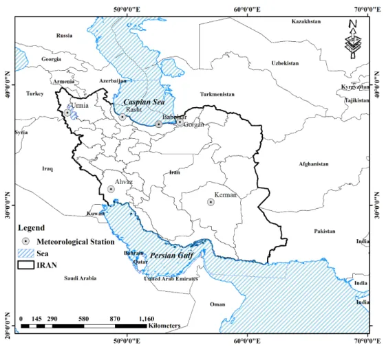
Iran, with an area of over 1648000 square kilometers, is located in the Northern Hemisphere and on the Asian continent. Iran, with an average annual precipitation of 250 mm, is located between the two meridians of 44° and 64°

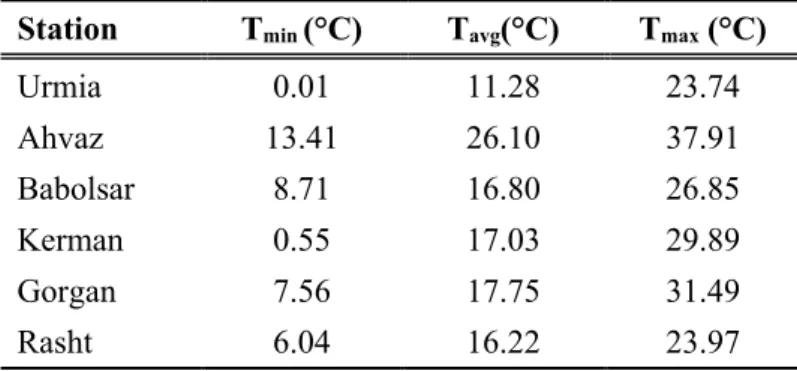
East and two circuits 25° and 40° North. About 94.8 percent of the country's surface area is located in arid and semi-arid regions with low precipitation and high evapotranspiration (Khalili et al., 2016). In this study, monthly minimum, maximum, and average air temperatures, saturation vapor pressure, actual vapor pressure, monthly precipitation, dew point temperature, and relative humidity of Babolsar, Gorgan, Kerman, Rasht, Urmia, and Ahvaz stations were used in a 64-year-long statistical period (1951–2014). Fig. 1 shows the studied area and the position of the stations. The characteristics of the meteorological stations were also described in Table 1.

Fig. 1. Location map of the selected stations in Iran.

Table 1. Annual statistics of stations used in the period 1951–2014 (°C) Tmax

(°C) Tavg

(°C) Tmin

Station

23.74 11.28

0.01 Urmia

37.91 26.10

13.41 Ahvaz

26.85 16.80

8.71 Babolsar

29.89 17.03

0.55 Kerman

31.49 17.75

7.56 Gorgan

23.97 16.22

6.04 Rasht

2.2. De Martonne climate factor

De Martonne proposed the following formula in 1926 with variations in the relationship and the replacement of the evaporation with temperature (Deer, 1963):

10

= + T

I P , (1)

whereI is the De Martonne aridity index, P is equal to the annual precipitation (mm), and T is equal to the average annual air temperature (°C). Although evaporation factor has been eliminated in De Martonne’s relationship, evaporation has also been related to air temperature and rising temperature, increases evaporation. Therefore, the high value of I can be high due to low air temperature or high precipitation. Based on De Martonne’s relationship, six types of climates have been classified in Table 2.

Table 2. Climatic classification based on the De Martonne index I Climate

I < 10 Dry

10 < I < 19.9 Moderately dry

20 < I < 23.9 Mediterranean

24 < I < 27.9 Moderately wet

28 < I < 34.9 Wet

35 < I Extremely wet

2.3. Support vector regression (SVR)

The first use of this model in water issues was presented by Dibike et al. in 2001 by precipitation-runoff modeling (Hofmann et al., 2002). The support vector machine (SVM) of an efficient learning system based on a theory of optimization must use the principle of inductive minimization of structural error and leads to a general optimal solution. In the SVM regression model, the function related to the dependent variable Y, which itself is a function of several independent variables x, is estimated (Eq. 2). Similar to other regression issues, the relationship between independent and dependent variables is determined with algebraic function f(x) (Eq. 3) plus allowed error ε:

( )

y f x= +noise, (2)

( )

^T

( )

f x =W .φ x +b (3)

If W (vector of coefficients) and b (constant) are the characteristics of the regression function and φ is a kernel function, then the goal is to find a functional form for f(x). This is accomplished by training SVM model by a set of samples (training set). Therefore, in order to calculate W and b, the error function must be optimized in the ε -SVM model, taking into account the conditions set out in Eqs. (4 and 5):

*

1 1

1 .

2

N N

T

i i

i i

W W C

ξ

C

ξ

= =

+

∑

+

∑

⁽⁴⁾

*

*

. ( ) . ( )

, 0 , 1,...,

T

i i i

T

i i

i

i i

W b

W b

i N

x y

y x

φ ε

φ ε

ξ ξ ξ ξ

+ − ≤ +

− − ≤ +

≥ =

(5)

In the above equations, C is a positive integer that determines the penalty when a model training error occurs, φ is the kernel function, N is the number of samples, and the two indices of

ξ

_i ^and

ξ

^*_i are the Slack variables, which determine the upper and lower limit of the training error associated with the allowed error value ε. In problems, it is predicted that the data is within the boundary range ε. Now, if the data is out of range ε, there will be an error equal to

ξ

_i ^and

ξ

^*_i . It is worth mentioning that the SVM model solves the problems

caused by the under fitting and over fitting by simultaneously minimizing two terms W W^T. / 2 and training errors, namely ^*

1( )

N

i i

i

C

ξ ξ

=

∑

+ , in. Therefore, by introducing the Lagrange coefficients

a

_i ^and

a

^*i , the optimization problem will be solved with numerical maximization of the following quadratic function (Eqs. 6 and 7):

* *

1 1

* *

, 1

( ) ( )

0.5 ( )( )

( ) ( )

N N

i i i i

i i i

N T

i i j j

i j i j

y a a a a a a a a x x

ε

φ φ

= =

=

+ − + −

+ +

∑ ∑

∑

^{, (6)}

* 1

*

( ) 0

0 , 0 , 1,2,...,

N

i i

i

i C i C i N

a a

a a

=

+ =

≤ ≤ ≤ ≤ =

∑

_{. (7)}

The above objective function is a convex function, and therefore, the solution would be unique and optimal. After defining the Lagrange coefficients, the characteristics w and b in the SVM regression model is calculated using the Karush-Kan-Tucker theory (Eq. 8):

* 1

( )

( )

N

i i

j

W ⁼

∑

₌

a a x

^{+ φ} i ^{. (8)}

As a result, the SVM regression model is:

* 1

( )

( ) (x)

N T

i i

i

W ⁼

∑

₌

a a x

^{+ φ} i ^{φ +}b^{. (9)}

It should be noted that the Lagrange terms ((

a a

_i^{+ *}_i)) can be zero or non- zero. Therefore, only data sets whose coefficients

a

_i are non-zero are entered in the final regression equation, and this data set is known as the support vectors.

In simple terms, support vectors are data that help to create a regression function. Among the vectors mentioned, those whose

a

_i values are less than C are called margin support vectors. When the value

a

_i of the support vectors is equal to C, it is known as an error support vector or a bounded support vector.

Margin support vectors are found on the margin of the insensitive boundary, while error support vectors are out of range. Finally, the regression SVM function can be rewritten in the following form:

1

( ) ^N i

( )

^T

( )

i

f x ⁼

∑

₌

a x

^φ i ^φ

x

j ⁺b^{. (10)}

In Eq. (10), the calculation of φ(x) in its characteristic space may be very complicated. To solve this problem, the regular trend in the SVM regression model is the selection of a kernel function as ^{K x x}( , )^{i =φ}

( ) x

_i ^{Tφ b2 −}4^{ac .} Various kernel functions can be used to construct different types of ε-SVM models. The most commonly used kernel functions available in the vector regression model are: (i) polynomial kernel with 3 target characteristics, (ii) a sigmoid kernel containing 2 target characteristics, and (iii) a kernel of radial base functions (RBF) with target characteristics.

2.4. Ant colony algorithm (ACO)

The ACO algorithm is a meta-exploration methodology that was proposed in 1992 by Dorigo. The ant colony algorithm was the first ACO algorithm proposed by Colorni et al. in 1991. One of the first applications of the ACO algorithm has been to solve the traveling salesman problem (Dorigo, 1992).

Since the ACO algorithms depend on the type of use and similarity of the ants moving on the graph, the use of the traveling salesman problem to explain the basic principles of ant algorithms was highly logical, and it was originally a typical example for introducing this algorithm (Akbarpour et al., 2020).

In this study, the ACO algorithm with 50 replicates and 50 members of the population was used to optimize the ε, sigma, and C parameters of the multivariate support vector regression (MSVR) model to develop the MSVR- ACO model. The objective function in the algorithm is to reduce the error rate in the estimated values using the root mean square error (RMSE).

In this study, different input patterns of meteorological data have been investigated as input of the MSVR-ACO model, and the superior model was determined at each meteorological station. The four patterns in this study are described in Table 3. The flowchart of the proposed methodology is demonstrated in Fig. 2.

Table 3. Patterns of the MSVR-ACO model

Pattern Number of inputs Input variables

I seven parameters monthly minimum, maximum, and average air temperatures, monthly precipitation, saturation vapor pressure, actual vapor pressure, and relative humidity II three parameters monthly average air temperature, saturation vapor

pressure, and actual vapor pressure

III two parameters monthly minimum and maximum air temperatures

IV one parameter monthly average air temperature

Fig. 2. Flowchart of the proposed methodology.

3. Results and discussion

As it was mentioned, the De Martonne’s method was used to study the climate in the studied areas. Results of the study are presented in Table 4.

Table 4. Results of the study of the climate of the studied areas based on the De Martonne index

Climate De Martonne

index Annual

precipitation (mm) Average annual air

temperature (^oC) Station

Moderately dry 15.85

337.33 11.28

Urmia

Dry 6.49

234.40 26.10

Ahvaz

Wet 33.24

890.88 16.80

Babolsar

Dry 5.45

147.53 17.03

Kerman

Mediterranean 20.59

571.53 17.75

Gorgan

Extremely wet 50.89

1334.51 16.22

Rasht

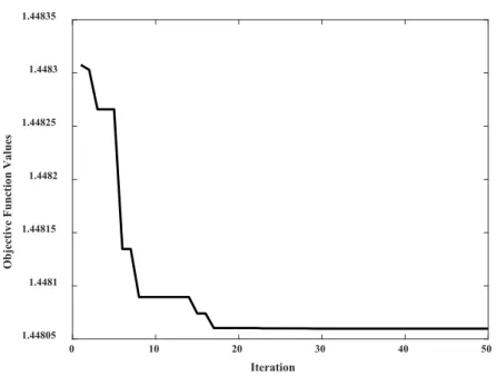
According to the results presented in Table 4, it can be seen that the stations studied have been selected from different climates. It should be noted that in this research the ACO algorithm was used to optimize the parameters of the MSVR model. The results of the evaluation of the performance of the ACO algorithm in estimating the DPT values of the Babolsar station were presented as an example in Fig. 3. Regarding Fig. 3, it can be seen that after 17 iterations, no improvement was achieved.

Fig. 3. Results of the performance of the ant colony algorithm in estimating DPT values at Babolsar station (Pattern IV).

0 10 20 30 40 50

Iteration 1.44805

1.4481 1.44815 1.4482 1.44825 1.4483 1.44835

Objective Function Values

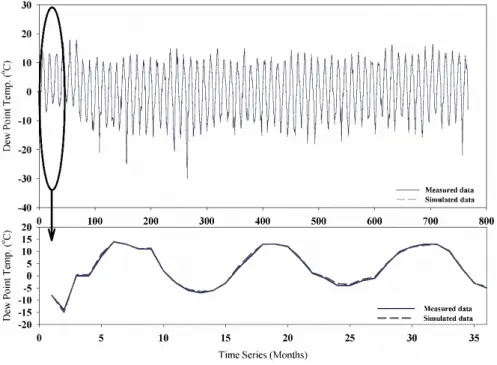
The DPT values was simulated using the optimal values of the parameters of the MSVR model. The results of estimating the DPT values of Gorgan and Kerman stations are presented in Figs. 4 and 5 (Pattern I)

Fig. 4. Estimation of DPT values of Gorgan meteorological station using Pattern I.

Fig. 5. Estimation of DPT values of Kerman meteorological station using Pattern I.

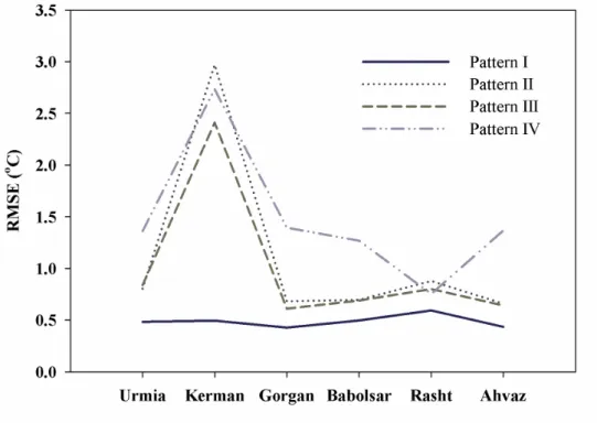
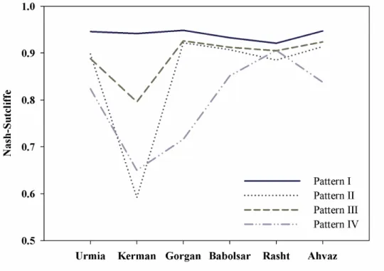
According to the results presented in Figs. 4 and 5, it can be seen that selection of seven parameters as inputs of the MSVR-ACO model will be able to model the DPT values of the studied stations. Also, the results indicate the DPT values with high accuracy, which have been derived from the integration of the MSVR model and the ACO algorithm. Other input patterns were also calculated, and the accuracy of different patterns were verified by three RMSE, coefficient of determination (R²), and Nash–Sutcliffe model efficiency coefficient tests. The results of the investigation and verification of various patterns in the estimation of DPT values are presented in Figs. 6, 7, and 8.

The results of verification of MSVR-ACO model in examining different patterns indicated that in Gorgan meteorological station, Pattern I had the lowest RMSE (Fig. 5). At this station, Pattern III was ranked second. This pattern has an RMSE of 0.61 °C in estimating DPT values. Pattern IV has error almost identical to a high RMSE, Pattern I, Pattern II, and Pattern III. In general, based on the RMSE, Pattern I is the best pattern followed by Pattern III, Pattern II, and Pattern IV respectively. The NSE coefficient also indicated that Pattern I and Pattern III have higher efficiency than Pattern II, and Pattern IV. The NSE model efficiency coefficient, as well as the RMSE, identified Pattern I, Pattern III, Pattern II, and Pattern IV as better patterns, respectively (Fig. 7). However, the performance of Pattern II and Pattern III is very similar to each other. Based on the R² between estimated and measured values, it was found that all patterns are highly correlated (Fig. 8). The Gorgan meteorological station is located in the mediterranean climate in terms of the De Martonne index, with an average temperature of 17.75 °C.

Fig. 6. Verification of different patterns in estimation of DPT values using RMSE.

Fig. 7. Verification of different patterns in estimation of DPT values using NSE.

Fig. 8. Verification of different patterns in estimation of DPT values using R².

At the Kerman meteorological station, Pattern I was introduced as a top model in estimating DPT values. According to the RMSE, Pattern I is the best pattern for estimating the DPT values of this station, which includes an error equal to 0.49 °C. After Pattern I, Pattern III has the lowest RMSE. Pattern II has the highest RMSE the Kerman station. Based on the RMSE, Pattern IV and Pattern II are assigned the third and fourth ranks with an error value of 2.73 and 2.97 °C, respectively. The NSE model efficiency coefficient also introduced Pattern I as the best pattern for estimating DPT values, and based on this criterion, as well as the RMSE, Pattern III was ranked as the second. Pattern IV and Pattern II were introduced as the third and fourth ranks in estimation of the DPT values.

The coefficient of R² also introduced Pattern I as the superior pattern and Pattern II as a worse pattern for estimating DPT values at Kerman station.

The Urmia meteorological station has a moderately dry climate with an average temperature of 11.28 °C. Based on the RMSE results in modeling the DPT values of this station, it was determined that Pattern I is the best pattern for estimating DPT values. Based on the RMSE values, Pattern II with an error value of 0.80 °C has the second rank. Patterns III and IV ranked as the third and fourth, respectively. The results show the same acceptable accuracy in Pattern II and Pattern III. In addition to the RMSE, the results of the NSE model efficiency coefficient showed that Pattern I and II are better. Based on the NSE model efficiency coefficient, Pattern III and IV were ranked as the third and fourth, respectively. The results of the coefficient of determination of the model also introduced Patterns I and II as superior patterns, which expresses the high accuracy of Patterns I and II compared to Patterns III and IV.

The wet station in this study is Babolsar station with an average temperature of 16.8 °C. Based on the RMSE, Pattern I was identified as the best. The RMSE value of Pattern I in the estimation of DPT values in Babolsar station is about 0.49 ° C.

Pattern III with the lowest RMSE has the second rank followed by Patterns II and IV.

There is not much difference between Pattern II and Pattern III. The NSE model efficiency coefficient also showed that Pattern IV has weak efficiency in modeling the DPT values of the Babolsar station, while Patterns III and II have a good performance in estimating DPT values. The accuracy of Patterns III and II was also confirmed according to the R² between measured and simulated data.

The meteorological station of Rasht with an average temperature of 16.22 °C is considered to be in the extremely wet regions of Iran in terms of the De Martonne climate index. Verification of DPT values at this station based on the RMSE showed that Pattern I is the best pattern for estimating DPT values and has the lowest RMSE (0.59 °C). The RMSE value in Pattern III is equal to 0.80 °C, and in Patterns II and IV it is 0.87 and 0.75 °C, respectively. The NSE model efficiency coefficient also considered the efficiency of Pattern I to be excellent in estimating DPT values. According to the NSE model efficiency coefficient, Pattern II was the worst. Patterns I, III, and IV have good efficiency.

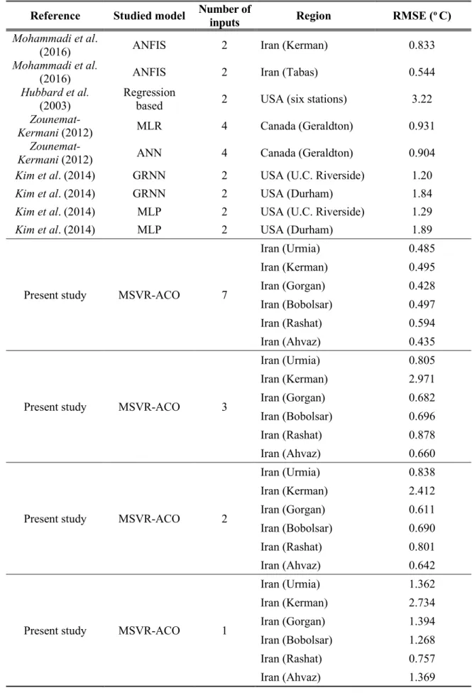
At Ahvaz meteorological station, Pattern I was introduced as the best pattern according to the three criteria of RMSE, NSE, and R². The RMSE ranked Pattern III as the second pattern. Patterns III and II have the same RMSE, approximately. The NSE model efficiency coefficient is also obtained with the values obtained from Patterns I, III, and II. These three patterns are presented as superior patterns in terms of efficiency. The coefficient of determination of the estimation of all patterns is high. In general, the results indicated that Pattern I was better at most stations as this has been confirmed by Mohammadi et al. (2016). According to the studies done on this topic in different regions, a comparison between the results of the models and the number of inputs has been made, and the results are presented in Table 5. The results of checking the RMSE values compared with the results of other researchers using two input parameters showed that, compared to Mohammadi et al. (2016), the accuracy of the ANFIS model was same as the MSVR model in the study area. Meanwhile, in other parts of the world, the accuracy of the MSVR-ACO model is proven to be higher than that of the other models.

4. Conclusion

One of the problems with estimating DPT values is the availability of many parameters. Therefore, the use of a model that can accurately estimate these (DPT) values with lower parameters is of great importance. Today, with the development of computer softwares and powerful processors, there are several methods and softwares available for estimating unavailable data and prediction.

These models include black box models of artificial neural network, ANFIS models, various algorithms, linear time series models, nonlinear models, and so on. Nevertheless, each of these types of models requires their own assumptions or is not suitable for any type of data. Also, the type of data input and the number of inputs are different for the models. In addition to the foregoing, a selection of data should also be made before modeling or predictions, so that better inputs with high correlation can be selected as inputs. In this study, meteorological data from six stations from different climates of Iran were used to estimate DPT values. To estimate DPT values, four patterns were used as inputs. Pattern I was selected with seven inputs, Pattern II with three inputs, Pattern III with two inputs, and Pattern IV with one input as study patterns. As it was mentioned above, non-linear MSVR-ACO model was used to estimate DPT values. Also, to optimize the parameters of the mentioned model, the ACO algorithm was used. In fact, in this study, DPT values were estimated using the MSVR-ACO combined model. The precision of estimated values at each station was investigated by the RMSE, NSE model efficiency coefficient, and R² methods.

Table 5. Comparison of the results of the present study with some existing researches

RMSE (^o C) Region

Number of inputs Studied model

Reference

0.833 Iran (Kerman)

2 ANFIS

Mohammadi et al.

(2016)

0.544 Iran (Tabas)

2 ANFIS

Mohammadi et al.

(2016)

3.22 USA (six stations)

Regression 2 based Hubbard et al.

(2003)

0.931 Canada (Geraldton)

4 Zounemat- MLR

Kermani (2012)

0.904 Canada (Geraldton)

4 Zounemat- ANN

Kermani (2012)

1.20 USA (U.C. Riverside)

2 GRNN

Kim et al. (2014)

1.84 USA (Durham)

2 GRNN

Kim et al. (2014)

1.29 USA (U.C. Riverside)

2 Kim et al. (2014) MLP

1.89 USA (Durham)

2 MLP

Kim et al. (2014)

0.485 Iran (Urmia)

7 MSVR-ACO

Present study

0.495 Iran (Kerman)

0.428 Iran (Gorgan)

0.497 Iran (Bobolsar)

0.594 Iran (Rashat)

0.435 Iran (Ahvaz)

0.805 Iran (Urmia)

3 MSVR-ACO

Present study

2.971 Iran (Kerman)

0.682 Iran (Gorgan)

0.696 Iran (Bobolsar)

0.878 Iran (Rashat)

0.660 Iran (Ahvaz)

0.838 Iran (Urmia)

2 MSVR-ACO

Present study

2.412 Iran (Kerman)

0.611 Iran (Gorgan)

0.690 Iran (Bobolsar)

0.801 Iran (Rashat)

0.642 Iran (Ahvaz)

1.362 Iran (Urmia)

1 MSVR-ACO

Present study

2.734 Iran (Kerman)

1.394 Iran (Gorgan)

1.268 Iran (Bobolsar)

0.757 Iran (Rashat)

1.369 Iran (Ahvaz)

The results showed that at almost all stations Pattern I was ranked first. In general, stations of Urmia, Kerman, Gorgan, Babolsar, Rasht, and Ahvaz, Pattern II has about 66, 500, 59, 40, 48, and 52 percent increased RMSE, respectively. Pattern III was recognized as a suitable pattern at all meteorological stations. The use of all of the seven parameters in the investigation and estimation of the DPT values of the stations under consideration will be highly accurate. However, the problem with the use of seven parameters will be as follows:

a) Receiving and collecting all the required informations is difficult and requires a lot of time.

b) Using all parameters in estimating DPT values reduces the computational speed and adjusts the computations to the algorithms to be considered.

c) Despite the availability of all the existing parameters, there is no need to use different models to estimate DPT values.

Therefore, the use of all of the seven parameters in the estimation of DPT values, which increases the accuracy of modeling, is not recommended. Based on the above mentioned results, it can be concluded that for each stations Pattern III (using the parameters of the monthly minimum and maximum air temperatures as model inputs), is a suitable pattern to estimate the monthly DPT values.

Acknowledgements: Authors are thankful to the University of Birjand, Birjand, Iran.

References

Akbarpour, A., Zeynali, M.J., and Tahroudi, M.N., 2020: Locating optimal position of pumping Wells in aquifer using meta-heuristic algorithms and finite element method. Water Resources Management. 34(1), 21-34.

Alvisi, S., Mascellani, G., Franchini, M., and Bardossy, A., 2006: Water level forecasting through fuzzy logic and artificial neural network approaches. Hydrol. Earth Syst. Sci. Discuss.10, 1–17.

https://doi.org/10.5194/hess-10-1-2006.

Citakoglu, H., Cobaner, M., Haktanir, T., and Kisi, O., 2014: Estimation of monthly mean reference evapotranspiration in Turkey. Water Res. Manage. 28, 99–113.

https://doi.org/10.1007/s11269-013-0474-1

Cobaner, M., Citakoglu, H., Kisi, O., and Haktanir, T., 2014: Estimation of mean monthly air temperatures in Turkey. Comput. Electron. Agricult.109, 71–79.

https://doi.org/10.1016/j.compag.2014.09.007

Colorni, A., Dorigo, M., and Maniezzo, V., 1991: Ant system: An autocatalytic optimizing process.

Dipartimento Di Elet-tronica, Politecnico Di Milano, Milan, Italy.

Doerr, A.H., 1963: De Martonne's Index of Aridity and Oklahoma's Climate. Proc. Oklahoma Acad.

Sci. 43, 211–213.

Dibike, Y.B., Velickov, S., Solomatine, D., and Abbott, M.B., 2001: Model induction with support vector machines: introduction and applications. J. Comput. Civil Engin.. 15, 208–216.

https://doi.org/10.1061/(ASCE)0887-3801(2001)15:3(208)

Dorigo, M., 1992: Optimization, learning and natural algorithms. PhD Thesis, Politecnico di Milano.

Dorigo, M., Maniezzo, V., and Colorni, A., 1991: Ant System: An Autocatalytic Optimizing Process Dip. Elettronica, Politecnico di Milano, Technical Report 91-016REV.

Govindaraju, R.S., 2000: Artificial neural networks in hydrology. I: Preliminary concepts.

J. Hydrol. Engin. 5, 115–123.https://doi.org/10.1007/978-94-015-9341-0

Hamel, L.H., 2011: Knowledge discovery with support vector machines. Vol 3. John Wiley & Sons.

Hofmann, T., Tsochantaridis, I., and Altun, Y., 2002: Learning over structured output spaces via joint kernel functions. In: Proceedings of the Sixth Kernel Workshop.

Hubbard, K.G., Mahmood, R.,and Carlson, C., 2003: Estimating daily dew point temperature for the northern Great Plains using maximum and minimum temperature. Agronomy J. 95,323–328.

https://doi.org/10.2134/agronj2003.3230

Imani, M., You, R.J., and Kuo, C.Y., 2014: Forecasting Caspian Sea level changes using satellite altimetry data (June 1992–December 2013) based on evolutionary support vector regression algorithms and gene expression programming. Glob. Planet. Change 121, 53–63.

https://doi.org/10.1016/j.gloplacha.2014.07.002

Jeong, C., Shin, J.Y., Kim, T., and Heo, J.H., 2012: Monthly precipitation forecasting with a neuro- fuzzy model. Water Res. Manage. 26, 4467–4483. https://doi.org/10.1007/s11269-012-0157-3 Khalili, K., Tahoudi, M.N., Mirabbasi, R., and Ahmadi, F., 2016: Investigation of spatial and temporal

variability of precipitation in Iran over the last half century. Stoch. Environ. Res. Risk Assess.

30,1205–1221. https://doi.org/10.1007/s00477-015-1095-4

Khan, M.S. and Coulibaly, P., 2006: Application of support vector machine in lake water level prediction. J. Hydrol. Engin. 11, 199–205. https://doi.org/10.1061/(ASCE)1084- 0699(2006)11:3(199)

Kim, S., Singh, V., Lee, C., and Seo, Y., 2015: Modeling the physical dynamics of daily dew point temperature using soft computing techniques. KSCE J. Civil Engin. 19, 1930–1940.

https://doi.org/10.1007/s12205-014-1197-4

Koza, J.R., 1992: Genetic Programming II, Automatic Discovery of Reusable Subprograms. MIT Press, Cambridge, MA.

Mohammadi, K., Shamshirband, S., Petković, D., Yee, L., and Mansor, Z., 2016: Using ANFIS for selection of more relevant parameters to predict dew point temperature. Appl. Thermal Engin.

96, 311–319. https://doi.org/10.1016/j.applthermaleng.2015.11.081

Pai, P.F. and Hong, W.C., 2007: A recurrent support vector regression model in rainfall forecasting.

Hydrol. Proc. 21, 819–827. https://doi.org/10.1002/hyp.6323

Ruan, J., Zhan, Q., Tang, L., and Tang, K., 2018: Real-Time Temperature Estimation of Three-Core Medium-Voltage Cable Joint Based on Support Vector Regression. Energies 11(6), 1405.

https://doi.org/10.3390/en11061405

Santamaría-Bonfil, G., Reyes-Ballesteros, A., and Gershenson, C., 2016: Wind speed forecasting for wind farms: A method based on support vector regression. Renew. Energy 85, 790–809.

https://doi.org/10.1016/j.renene.2015.07.004

Shiri, J., Kim, S., and Kisi, O., 2014: Estimation of daily dew point temperature using genetic programming and neural networks approaches. Hydrol. Res. 45,165–181.

https://doi.org/10.2166/nh.2013.229

Vapnik, V., 1998: Statistical learning theory Wiley, New York.

Zounemat-Kermani, M., 2012: Hourly predictive Levenberg–Marquardt ANN and multi linear regression models for predicting of dew point temperature. Meteorol. Atmosph. Phys. 117, 181–192.

https://doi.org/10.1007/s00703-012-0192-x