DOI:10.28974/idojaras.2020.2.7
IDŐJÁRÁS
Quarterly Journal of the Hungarian Meteorological Service Vol. 124, No. 2, April – June, 2020, pp. 277–297
Validating AquaCrop model for rainfed and irrigated maize and soybean production in eastern Croatia
Monika Marković1*, Marko Josipović2, Milena Jančić Tovjanin3, Vladimir Đurđević4, Marija Ravlić1, and Željko Barač1
1University of Josip Juraj Strossmayer in Osijek Faculty of Agrobiotechnical sciences Osijek
Vladimira Preloga 1, Osijek, Croatia
2Agricultural Institute Južno predgrađe 17, Osijek, Croatia
3University of Novi Sad Faculty of Agriculture
Novi Sad, Serbia
4University of Belgrade
Faculty of Physics Institute of Meteorology Dobracina 16, Beograd, Serbia
*Corresponding Author e-mail: monika.markovic@fazos.hr (Manuscript received in final form April 30, 2019)
Abstract⎯ In this study, the AquaCrop model was used to quantify climate change impact on yield and net irrigation in maize and soybean production. Daily observed climate data (1961–1990) from Osijek weather station were used for past climate simulation, and output data from ECHAM model were dynamically downscaled under two IPCC SRES scenarios (A1B, A2) for two integration periods 2041–2070 and 2071–
2100. The soil properties and crop data were presented from 6-year-long (2010–2015) field study of the Agricultural Institute in Osijek, Osijek-Baranja County. The climate results showed expected rise in air temperature up to 5 ºC and significantly lower precipitation up to 43.5%. According to results from the AquaCrop model, there is no change in maize yield in non-irrigated conditions, while in irrigated conditions there is a yield increase of 1.4 t ha-1 of dry matter (dm), with 80 mm higher net irrigation in comparison with the 1961–1990 period. As for soybean production, the increase in yield is expected in both non-irrigated and irrigated conditions. The yield increases up to 1.9 dm t ha-1 in irrigated conditions with 90 mm higher net irrigation in comparison with the 1961–1990 period. As for crop water indices, in non-irrigated conditions the water use efficiency (WUE) has a trend to decrease in the future, while in irrigated conditions it can slightly increase. Irrigation water use efficiency (IWUE) showed significantly higher increase in irrigated maize and soybean production.
1. Introduction
Farms in Croatia can be characterized as considerably smaller than the EU average (14.4 ha) considering that the average farm size is 5.6 ha per holding, where one half of holdings are less than 2 ha (Eurostat, 2017). This fact is one of the most important specific restrictive effects on expansion of irrigation areas in Croatia. According to the recent published official data, in Croatia only 13,430 ha (1.4% of arable lands) is irrigated (MEE, 2014). In the Osijek-Baranja County, the study region, total equipped area for irrigation is 1,390 ha, whereby 512 ha with groundwater, while 878 ha with surface water (Crostat, 2006).
Future expansion of irrigation areas in Croatia is encouraged by government and policy measures, so the goal is to provide infrastructure to implement irrigation on 65,000 ha of arable lands until the year 2020 (Holjević et al., 2008). In Croatia, irrigation is manly used on supplementary basis to improve production of summer crops. Above 56% of agricultural areas in Croatia are categorized as arable lands, while in Osijek-Baranja County nearly 95% (200892 ha). Total agricultural land in Osijek-Baranja County is 212,095 ha, whereby 200,892 ha is arable land. In average 60.8% of arable lands are sown with maize, while 14.6%
with soybean. The considerable yield variation of summer crops is mainly caused by unfavorable weather conditions. Not only because of the lack of rainfall but because of the dry periods which prolonged for fifteen years, local authorities proclaimed natural disaster of drought (2000, 2003, 2007, 2011, 2012, 2013, and 2015). According to Perčec Tadić et al. (2014) among all natural hazards in Croatia, drought causes the largest economic losses (39%). A more detailed analysis of drought phenomena in the Republic of Croatia have been done by Cindrić et al. (2016). Authors claim that the examined 2011/2012 drought in Osijek-Baranja County was characterized by extremely long duration with the highest magnitudes since the beginning of the twentieth century.
Branković et al. (2009) have stated that during the twentieth century, the decline in annual amounts of precipitation in Osijek area is –4.1% in spring and –3% in autumn. As a result, in dry growing seasons, the yields of main summer crops grown in farm conditions are reduced as follows (CBS, 2018): maize yield was reduced by 39.7% (2010), 38.3% (2003), 28% (2007), 1.2% (2011), 22.1%
(2012), 4.5% (2013), and 4.2% (2015), while soybean yields were reduced by 41.7% (2010), 29.3% (2003), 20.8% (2007), 25% (2013), and 8.3% (2015).
Therefore, the importance of irrigation practice in this region is unquestionable.
Furthermore, the yields of summer crops in several field studies are considerably increased by compensating the lack of rainfall with irrigation water. Some previously published results have evaluated the effect of irrigation treatments on maize yield in the study region. For example, in full irrigated plots, which was set to achieve soil water content of 80 to 100% of field capacity (FC), maize yield was by 25% (2011) and by 40% (2012) higher compared to control (dryland) plots (Marković et al., 2015). As for soybean, in full irrigated plots
yields were by 9.4% (2007), 12.2% (2009), 46% (2012), and 18.8% (2013) higher compared to control plots (Josipović et al., 2011, 2013). The irrigation efficiency (IE) is usually interpreted as the yield increase or reduction in irrigated agriculture. According to Irmak et al. (2011), irrigation efficiency (IE) is generally defined from three points of view: (1) the irrigation system performance, (2) the uniformity of water application, and (3) the response of the crop to irrigation. Some DSSAT crop simulations were done in term of climate changes and influence on maize production, and it was shown that in the future Croatia would belong to the area of decreased maize yields (Vučetić, 2008). The maize yield was simulated in non-irrigated conditions. This research emphasizes the importance of adaptation for summer crop production in terms of implementation of irrigation practice. The AquaCrop model was chosen in this paper to simulate the non-irrigated and irrigated production as the adequate and ideal crop model for irrigation evaluation, developed by Food and Agriculture Organisation of United Nation (FAO). According to Farahani et al. (2009), the FAO AquaCrop model provides a theoretical framework to investigate crop yield response to environmental stress, especially water and salinity. It simulates soil water balance and crop growth processes, based on input parameters and data, as a function of climate, soil, and plant interaction (Foster et al., 2017).
The model precisely simulates the crop production, as it operates on a daily input data. In literature, AquaCrop model is well known in research community and successfully validated through many regions and various crops for field production: wheat (Rezaverdinejad et al., 2014), maize (Ahmadi et al., 2015;
Paredes et al., 2014; Stricevic et al., 2011), sugar beet (Stričević et al., 2014), and sunflower (Todorovic et al., 2009) crop production. The aim of this paper was to validate the AquaCrop model in non-irrigated and irrigated maize and soybean production for climate and soil conditions of Osijek-Baranja County (eastern Croatia). In the next step, the AquaCrop model was used to simulate maize and soybean production for future climate conditions for the 2041–2070 and 2071–2100 periods. Further results are presented: (a) the relative change in yield of maize and soybean in non-irrigated and irrigated conditions; (b) the change in net irrigation, water use efficiency (WUE), and irrigation water use efficiency (IWUE).
2. Materials and methods 2.1. Location
The field study was conducted at the research site of the Agricultural Institute in Osijek (45º32'N and 18º44'E). The area of Osijek (Osijek-Baranja County, eastern Croatia) has an altitude of 90 m. According to the Köppen climate
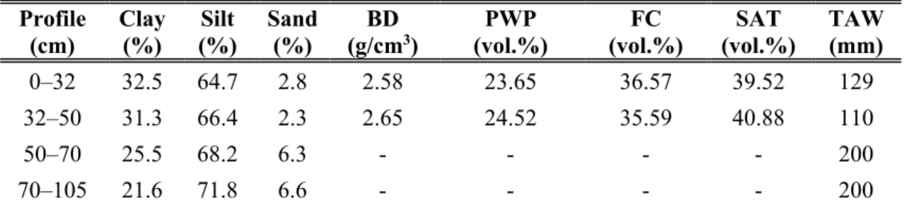
average air temperature of 10 ºC, and an annual sunshine of 4649 h. Mentioned climate data are expressed as an average for the 1961–1990 period. The soil is classified as gleysol (hydro-meliorated) WRB with its main characteristics presented in Tables 1 and 2. The soil analyses included mechanical, chemical, and soil water characteristics, sampled in two to four profile depth.
Table 1. Mechanical and hydrological characteristics of the soil at the research site Profile
(cm)
Clay (%)
Silt (%)
Sand (%)
BD (g/cm3)
PWP (vol.%)
FC (vol.%)
SAT (vol.%)
TAW (mm)
0–32 32.5 64.7 2.8 2.58 23.65 36.57 39.52 129
32–50 31.3 66.4 2.3 2.65 24.52 35.59 40.88 110
50–70 25.5 68.2 6.3 - - - - 200
70–105 21.6 71.8 6.6 - - - - 200
BD = bulk density; PWP = permanent wilting point; FC = field capacity; SAT = saturation;
TAW = total available water
Table 2. Chemical characteristics of soil at the research site Profile
(cm)
Organic carbon (%)
Nitrogen (%)
0–40 0.91 0.13 40–95 0.77 0.13
2.2. Past and future climate data
The past climate (1961–1990) presents daily weather data, observed at the weather station Osijek (45º32'N and 18º44'E) located nearby the experimental field. The data set includes maximum and minimum air temperature (ºC), insolation (h), precipitation (mm), vapor pressure (mbar), and wind speed (m/s).
The reference evapotranspiration was calculated applying the FAO Penman- Monteith method (Allen et al., 1998). For the future climate conditions, the data were assumed from the integrated coupled model ECHAM, developed at the Max Planck Institute for Meteorology (Roeckner et al., 2003). The modeled data
were dynamically downscaled for two periods: from 2041 to 2070 and from 2071 to 2100. All simulations were done under the A1B and A2 (IPCC, 2001) scenarios for greenhouse gas (GHG) emissions for two the integration periods mentioned above, considering CO2 effect. The average CO2 concentration was 333.4 ppm for the 1961–1990 period, 545.7 mm (A1B scenario) and 551.0 ppm (A2 scenario) for the 2041–2070 period, and 662.4 ppm (A1B scenario) and 731.1 ppm (A2 scenario) for the 2071–2100 period.
2.3. Field study and crop management
Maize and soybean yield data, presented in this paper, were observed from a long-term field experiment for the 2010–2015 period. For the purpose of this study, yield data are presented for maize hybrids FAO 500 and 600, and soybean varieties 0–1 group. The region and field plots as well as the crop management were previously presented by Josipović et al. (2013) and Marković et al. (2017).
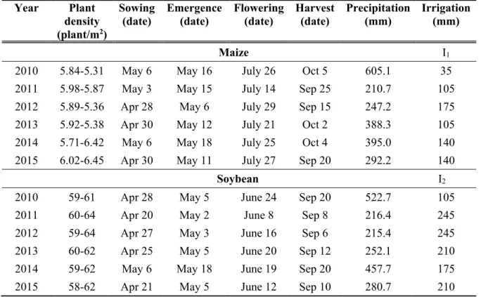
Planting date, density, as well as observed phenology (sowing, emergence, flowering, and maturity) are presented in Table 3. The size of the maize hybrid plot was 19.6 m2. Each year, maize hybrids were planted at 0.7 m row spacing, 0.25 m inter-row spacing, and depth of approximately 5 cm. The size of the soybean variety plot was 30 m2. Seeding density for soybean crop was 550 seeds/m2. Grain yield for both crops was measured after harvesting of each experimental plot, adjusted to 14% grain moisture and expressed as kg ha-1.
Since the maize and soybean yield data for this study are expressed for irrigation treatment, here follows a more detailed description of the irrigation scheduling. Studied irrigation treatments included dryland (I0-control) in both crop production, while the irrigated plot was designed to irrigate at 60–80%
field water capacity (FWC) for maize (I1) (Hoogenboom et al., 2012) and 80–
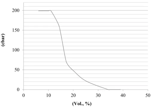
100% FWC (I2) for soybean, which is more vulnerable on the deficit in soil moisture. The size of irrigation plots for maize crop was 78.4 m2, while for soybean it was 120 m2. Irrigation was scheduled with the use of Watermark soil moisture sensors (model 200SS). The sensors were set up at two depths (15–20 cm and 25–30 cm) after the maize and soybean sowing, and were kept in soil until the harvest time. The Watermark sensors were calibrated for the soil on a trial site by comparing gravimetric measurements and sensor readings (Marković, 2013). The calibration curve is presented in Fig. 1. The maize and soybean were irrigated by use of traveling sprinkler system, which performed at the average speed of 15 m h-1 and provided 35 mm of irrigation water (1.5 l min-1).
Total amounts of water added in each growing season and irrigation treatments are presented in Table 3. Water for the system was pumped from 37 m deep well at a 5 to 7 l s-1 flow rate using an electric pump (5.5 kW). The analysis of chemical quality of irrigation water showed that the composition and concentrations of salts do not induce toxicity problems. The analysis was
interpreted according to FAO standards (Ayers and Westcot, 1985). The irrigation water use efficiency (IWUE) was determined as
= – , (1)
where IWUE is the irrigation water use efficiency (kg m-3), Yd is the yield (kg) on dry plots, Yi is the yield (kg) on irrigated plots, and I (m3) is the net irrigation water (Nakayama et al., 1979). The water use efficiency (WUE) was determined as
= / , (2)
where WUE is the water use efficiency (kg m-3), Y is the economic yield (kg m-3) for irrigation level, and ET0 (m3) is the reference crop evapotranspiration (Kang et al., 2000). The reference crop evapotranspiration (ET0) was calculated according to the Penman-Montheith method by using the AquaCrop model.
Fig. 1. Calibration curve of the Watermark sensors for the soil type at the study site.
(Marković, 2013) 0 50 100 150 200
0 10 20 30 40 50
(cbar)
(Vol., %)
Table 3. Planting date, density, and observed phenology for maize and soybean crops Year Plant
density (plant/m2)
Sowing (date)
Emergence (date)
Flowering (date)
Harvest (date)
Precipitation (mm)
Irrigation (mm)
Maize I1
2010 5.84-5.31 May 6 May 16 July 26 Oct 5 605.1 35 2011 5.98-5.87 May 3 May 15 July 14 Sep 25 210.7 105 2012 5.89-5.36 Apr 28 May 6 July 29 Sep 15 247.2 175 2013 5.92-5.38 Apr 30 May 12 July 21 Oct 2 388.3 105 2014 5.71-6.42 May 6 May 18 July 25 Oct 4 395.0 140 2015 6.02-6.45 Apr 30 May 11 July 27 Sep 20 292.2 140
Soybean I2
2010 59-61 Apr 28 May 5 June 24 Sep 20 522.7 105 2011 60-64 Apr 20 May 2 June 8 Sep 8 216.4 245 2012 59-64 Apr 27 May 3 June 16 Sep 6 215.4 245 2013 60-62 Apr 25 May 5 June 20 Sep 12 252.1 210 2014 59-62 May 6 May 18 June 19 Sep 20 457.7 175 2015 58-62 Apr 21 May 5 June 12 Sep 10 280.7 210
2.4. Data analyses
Two statistical methods were used to analyze, evaluate, and compare observed yield data from field experiments and simulation yield results, to measure the AquaCrop model goodness of fit in our environmental conditions. First the relative deviation (Törnvist et al., 1985) was calculated between the simulated and observed dry matter yields for each year. The method was chosen to show how the model works and its sensitivity to various climate conditions each year under the same or similar crop management activity:
=
( )( ) , (3)
where r is the relative deviation (%), M is the observed yield (dm t ha-1), and S is the simulated yield (dm t ha-1). The crop model fits when r is less than 15%
(Tsuji et al., 1998). The second method selected for quantitative summary of goodness of fit was the root mean square error (RMSE):
= ∑ ( − ) , (4)
where RMSE is the root mean square error (dm t ha-1), yi is measured value, ŷi is the corresponding simulated value, and n is the number of measurements (Wallach et al., 2018). The RMSE has the same unit as the measured value y.
2.5. AquaCrop model, input data, calibration, and validation
The AquaCrop model is developed by FAO to simulate the crop response on the environmental stress. It is described by Steduto et al. (2009) in details. The model calculates daily biomass based on daily transpiration data, using reference evapotranspiration (ET0), and normalized water productivity. The simulated yield is calculated as the product of daily biomass using the harvest index (HI).
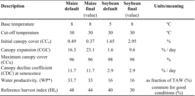
As the water is of the main importance in the AquaCrop model, it also simulates the changes in the soil water content during the growing season by means of a soil water balance. The soil water balance consists of the incoming water (rainfall, irrigation, and capillary rise), and outgoing water (runoff, evapotranspiration, and deep percolation) contained in different profiles of soil root zone depth. The moment for irrigation is possible to be calculated in the model, as the fixed amount of water retained and depleted in the root zone at any moment of the season. That possibility gives an opportunity to simulate irrigation efficiency on crop productivity (Greaves and Wang, 2017). To safely use simulation results by the AquaCrop model, it is necessary to do local calibration and validation for the chosen crop. The model requires a relatively small number of input data which describes the soil–crop–weather environment in which the crop develops (Stricevic et al., 2011). Using input data, observed daily weather data, soil characteristics, field management data, and crop parameters, the AquaCrop model was calibrated for maize and soybean production. For maize production, the model version 5.0 provides files with parameters suitable for the simulation of maize production, but with default values. These values were chosen only as a starting point, then the final key parameters were modified to fit the local crop management. All crop parameters were calibrated for the FAO 500–600 type maize hybrids, so that the crop model may simulate and present the real crop production in our local conditions. In Table 4 final parameters are given, which are used for AquaCrop model calibration for maize and soybean production. Initial canopy cover was 0.37%
with maximum canopy cover 96% in maize production (Table 4). The base air temperature was set to 8 ºC and the upper temperature to 30 ºC. Water productivity was 33 g m2 and harvest index was 44% (Table 4). The crop management was standard for our agro-ecological conditions for maize and soybean growing. Soil fertility was considered as sufficient to achieve an ideal yield genetic potential, thus we could estimate only the effects climate change conditions. Net irrigation for maize and soybean is presented in Table 3. The AquaCrop model was calibrated for maize production for year 2010, results are and shown in Table 5. The relative deviation between the non-irrigated observed
and simulated dry matter yields was 3%, and it was 3.9% between the irrigated observed and simulated yields. The absolute change for net irrigation was 20.7 mm.
Table 4. Default and final parameters for the Aquacrop model calibration for maize and soybean production
Description Maize default
Maize final
Soybean default
Soybean
final Units/meaning
(value) (value)
Base temperature 8 8 5 8 ºC
Cut-off temperature 30 30 30 30 ºC
Initial canopy cover (CCo) 0.49 0.37 1.65 2.95 % Canopy expansion (CGC) 16.3 23.1 1.6 9.6 % / day Maximum canopy cover
(CCx) 96 96 98 98 %
Canopy decline coefficient
(CDC) at senescence 11.7 11.7 2.9 2.9 % / day
Water productivity. (WP*) 33.7 33 16 16 as fraction of TAW (%) Reference harvest index (HIo) 48 44 40 30 common for good
conditions (%)
Table 5. Calibration (2010) and validation of maize grain yield (dm t ha-1) for the 2010–2015 period
Non irrigated Irrigated
Year
Observed yield (dm t ha-1)
Simulated yield (dm t ha-1)
Relative deviation
(%)
Observed yield (dm t ha-1)
Simulated yield (dm t ha-1)
Relative deviation
(%)
2010 7.9 7.7 -2.5 7.9 7.6 -3.9
2011 6.4 7.0 9.4 7.6 7.7 1.8
2012 6.4 5.7 -10.9 7.7 7.8 0.8
2013 7.4 6.9 -6.8 7.2 7.5 3.8
2014 10.5 7.8 -25.7 11.9 7.8 -34.2
2015 7.4 6.8 -8.1 9.3 7.8 -16.5
The validation was done for a six-year period from 2010 to 2015, at the same location (Table 5). The relative deviation between simulated and observed dry matter yields was calculated for each year according to Törnvist et al. (1985) indicating how model fits in various climate conditions under the same crop management. The relative deviation between non-irrigated simulated and observed yields varied from 3 to 11%, while in irrigated conditions from 0.8 to 16.5%, except in year 2014. The absolute change in net irrigation varied from 2.3 to 38.8 mm, except for 2014. The highest deviation in yield as well as the absolute change in net irrigation (93.9 mm) occurred in 2014. In that year, the number of rainy days was above the long-term average, with very significant higher precipitation at the end of the growing season.
This significant difference between simulated and observed yield values is a consequence of the model inability to simulate the plant reaction to stress in extreme conditions, such as high variations in daily air temperature and precipitation sum in short time intervals (Lalic et al., 2011). The second method selected for quantitative summary of goodness-of-fit was the RMSE method (Wallach et al., 2018). For the 5-year-long period (without the extreme weather year, 2014), it was 0.3 dm t ha-1 under non-irrigated maize production and 0.4 dm t ha-1 under irrigated maize production. The RMSE value was below 0.5 dm t ha-1 and showed that the model fits under our environmental conditions. The AquaCrop model was also calibrated for soybean 0 to 1 maturity group variety for year 2011 (Table 6). The relative deviation between non-irrigated simulated and observed dry matter yields was 1% and 3.8% in irrigated conditions. Absolute change for net irrigation was 3.2 mm. The model was validated for the 6-year-long experiment at the same experimental field (Table 6). The relative deviation between simulated and observed yields varied from 0 to 9% in non-irrigated conditions and from 0.4 to 5.1% in irrigated conditions, except in year 2010, when the relative deviation was 22 and 25.2%, due to heavy precipitation. The absolute change for net irrigation varied from 1.6 to 30 mm, except in year 2014, when the precipitation was considerably higher than the long-term average at the end of the growing season.
The RMSE for 6-year-long period was 0.07 dm t ha-1 under non-irrigated conditions and 0.09 dm t ha-1 under irrigated conditions, which improves the model validation under our environmental conditions.
To estimate the climate change impact on yield, net irrigation, and WUE in future conditions, it is necessary to keep same crop management operations and crop parameters in model as in the period of 2010–2015. The crop parameters and phenology stages, which were kept the same for the 1961–1990 period and future conditions are presented in Table 7. In the model, sowing and phenology were set at the average sowing date, emergence, maximum canopy cover, flower appearance and maturity date (Table 7). Additionally, under irrigated conditions, the readily available water was set to 80%, below which the soil water content in the root zone may not drop. This irrigation method in the model, including defined and set local soil hydrological characteristics, gave similar net irrigation quantities to measured net irrigation from field experiments.
Table 6. Calibration (2011) and validation of I group maturity soybean grain yield (dm t/ha) for the 2010 to 2015 period
Non irrigated Irrigated
Year
Observed yield (dm t ha-1)
Simulated yield (dm t ha-1)
Relative deviation
(%)
Observed yield (dm t ha-1)
Simulated yield (dm t ha-1)
Relative deviation
(%)
2010 2.9 3.5 22 2.8 3.5 25.2
2011 3.0 3.0 -1 3.9 3.7 -3.8
2012 2.4 2.5 5 3.7 3.7 -0.4
2013 2.9 2.9 0 3.8 3.7 -4.2
2014 3.1 3.3 7 3.5 3.7 5.1
2015 2.7 2.9 9 3.8 3.8 -1.4
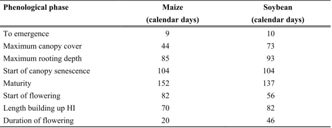
Table 7. Calendar days of maize and soybean by phenological phases for crop simulations for the 1961–1990 period and expected climate conditions
Phenological phase Maize Soybean
(calendar days) (calendar days)
To emergence 9 10
Maximum canopy cover 44 73
Maximum rooting depth 85 93
Start of canopy senescence 104 104
Maturity 152 137
Start of flowering 82 56
Length building up HI 70 82
Duration of flowering 20 46
3. Results 3.1. Past and future climate conditions
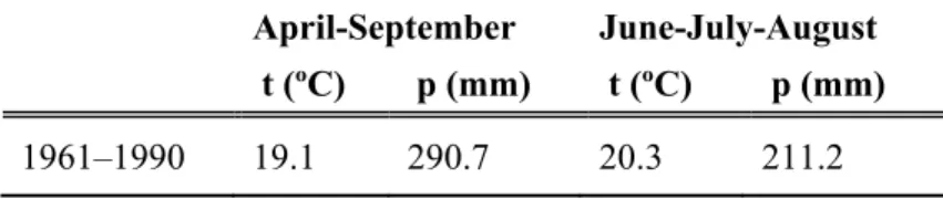
In the 1961–1990 period, the observed data were analyzed: air temperature and precipitation in the growing season AS (from April to September) and the drought period JJA (from June to August) (Table 8). The temperature was
was 290.7 mm for the growing season and 211.2 mm for JJA period (Table 8).
For future conditions, the absolute change in temperature and relative change in precipitation was calculated for the 2041–2070 and 2071–2100 periods under two scenarios (A1B, A2) in compare to 1961–1990 (Table 9). In future conditions, rise in temperature in both periods under two scenarios is expected.
There was no significant difference between the two scenarios from 0.3 to 0.5 ºC. In the AS period, the expected increase in temperature for the 2041–2070 period is 2.8 ºC (A1B) and for 2071–2100 is 4.6 ºC (A2). In the JJA drought period, the expected increase in temperature is 2.9 ºC (A1B) in 2041–2070 and 5.0 °C (A2) in 2071– 2100 (Table 9). The analyzed precipitation amount showed a significant decrease in future conditions compared to the past climate data of the period 1961–1990. In a comparison of the two scenarios, the A1B scenario showed lower precipitation for future conditions, especially for the 2041–2070.
In AS period, for 2041–2070, lower precipitation by 28.2% (A1B) and 16.5%
(A2) is expected. In the 2071–2100 period, more decrease in precipitation is expected, by 34.8% (A1B) and 33.7% (A2) in AS compared to 1961–1990.
During JJA summer months, a considerable decrease in precipitation is expected as well. In the 2041–2070 period, the expected reduction in precipitation is 35.2% (A1B) and 25.8% (A2). Furthermore, for the 2071–2100 period, 43.55%
(A1B) and 43.4% (A2) reduction is expected compared to the 1961–1990 period (Table 9).
Table 8. Climate conditions for the 1961–1990 period at Osijek location (t - temperature;
p - precipitation)
April-September June-July-August t (ºC) p (mm) t (ºC) p (mm)
1961–1990 19.1 290.7 20.3 211.2
Table 9. Absolute change in temperature (°C) and relative change in precipitation (%) for 2041–2070 and 2071–2100 using ECHAM model under A1B and A2 scenarios (t - temperature; p - precipitation)
A1B A2
April- September June-July-August April- September June-July-August t (°C) p (%) t (°C) p (%) t (°C) p (%) t (°C) p (%) 2041–
2070 2.8 -28.2 2.9 -35.2 2.3 -16.5 2.4 -25.8
2071–
2100 4.3 -34.8 4.5 -43.5 4.6 -33.7 5.0 -43.4
3.2. Climate change impact on maize and soybean yields, net irrigation, WUE, and IWUE
In past climate conditions (1961–1990), the simulated maize yield in non- irrigated conditions was as usual in real conditions, about 7.3 dm t ha-1, and 7.1 dm t ha-1 in irrigated conditions (Tables 10 and 11). For the same period of time, the WUE ranged from 1.32 kg m3 in non-irrigated to 1.28 kg m3 in irrigated conditions. As for IWUE, net irrigation (40 mm) reduced the maize yield for 3.53 kg mm-1. According to the analyzed yield results, in future conditions it is expected a little lower or the same yield in non-irrigated maize production, and higher yield values when the maize is under irrigated conditions (Tables 10 and 11). In the 2041–2070 period, in non-irrigated conditions, the maize should have 0.4 dm t ha-1 lower (A1B) or 0.2 dm t ha-1 (A2) higher yield.
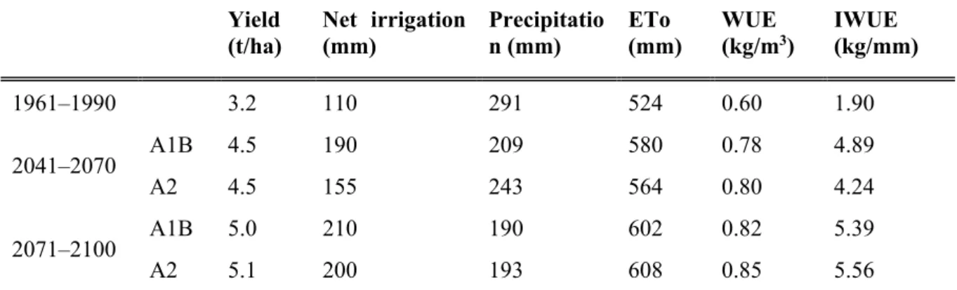
During the same period, the WUE for non-irrigated conditions for A1B scenario is 1.14 kg m3 and 1.28 kg m3 for A2 scenario. In the further period, till 2100, it is expected that the yield slightly decrease from 0.6% (A1B) to 0.3% (A2) compared to the 1961–1990 period. Furthermore, the WUE for this period is 1.07 kg m3 for A1B and 1.11 kg m3 for A2 scenario (Table 10). In irrigated conditions, maize production showed an increase in yield from 1.0 dm t ha-1 in 2041–2070 and 1.4 dm t ha-1 in 2071–2100. There were no significant differences between the results of the two scenarios. In irrigated conditions, it is important to mention that the net irrigation is expected to increase in both periods. In 2041–2070, the absolute change in net irrigation was 74.8 mm (A1B) and 38.3 mm (A2). For 2041–2070, the WUE is 1.34 kg m3 and IWUE is 11.8 kg mm for A1B scenario while for the A2 scenario WUE is 1.37 kg m3 and IWUE is 7.64 kg m3 (Table 11). In 2071–2100, further increase in net irrigation up to 80.7 mm under A2 scenario is expected. For this period, WUE is 1.33 kg m3 for both scenarios, while IWUE is 14.01 kg mm for A1B and 12.16 kg mm for A2 scenario. In soybean production, the crop simulations for the 1961–1990 period showed, that soybean yield was similar to real yield produced in Croatia, 2.9 dm t ha-1 in non-irrigated conditions and 3.2 dm t ha-1 in irrigated conditions (Tables 12 and 13). As for WUE, it ranges from 0.56 kg m3 in non-irrigated to 0.60 kg m3 in irrigated soybean production, while the IWUE was 1.9 kg mm. In future conditions, in both periods yield increase is expected. In 2041–2070, in non-irrigated production, the expected increase is from 0.7 (A1B) to 0.9 dm t ha-1 (A2) in soybean yield, while the larger increase is expected in the period 2071–
2100, for 0.9 dm t ha-1 under A1B scenario and 1.1 dm t ha-1 under A2 scenario.
The WUE, for the mentioned period, ranged from 0.61 to 0.68 kg m3 for A1B and A2 scenarios for 2041–2070, and from 0.63 to 0.66 kg m3 in 2071–2100 (Table 12). The rise in soybean yield in irrigated conditions is also noticeable, 1.3 (A1B) and 1.8 dm t ha-1 (A2) in the 2041–2070 period and 1.3 (A1B) to 1.9 dm t ha-1 (A2) in the 2071–2100 period. There was no significant difference
WUE is 0.6 kg m3, while IWUE is 1.9 kg mm (Table 13). In irrigated production, the net irrigation was significantly higher in both periods, than in the 1961–1990 period. The absolute change in net irrigation is expected to be 82.9 (A1B) and 46.3 mm (A2) in the 2041–2070 period and 103.5 (A1B) 93.3 mm (A2) in the 2071–2100 period. The WUE for the 2041–2070 period ranges from 0.78 to 0.80 kg m3 for A1B and A2 scenarios. Furthermore, for the 2071– 2100 period it ranges from 0.82 to 0.85 kg m3. As for IWUE for the 2041–2070 period, it ranges from 4.89 to 4.27 kg mm for A1B and A2 scenarios, while for the 2071–
2100 period it ranges from 5.39 to 5.56 kg mm for A1B and A2 scenarios (Table 13).
Table 10. Average yield (dm t/ha) and water use efficiency (WUE, kg/m3) for non- irrigated maize crop in 1961–1990 and future conditions under A1B and A2 SRES scenarios
Period Yield
(dmt/ha)
Precipitation (mm)
ETo (mm)
WUE (kg/m3)
1961–1990 7.3 313 551 1.32
2041–2070 A1B 6.9 220 607 1.14
A2 7.5 205 629 1.28
2071–2100 A1B 6.7 260 591 1.07
A2 7.0 206 637 1.11
A1B; A2 = scenarios, WUE = water use efficiency
Table 11. Average yield (dm t/ha), water use efficiency (WUE, kg/m3) and irrigation water use efficiency (IWUE, kg/mm) for irrigated maize crop in 1961-1990 and future conditions under A1B and A2 SRES scenarios
Yield (dmt/ha)
Net irrigation (mm)
Precipitation (mm)
ETo (mm)
WUE (kg/m3)
IWUE (kg/mm)
1961–1990 7.1 40 313 554 1.28 -3.53
2041–2070 A1B 8.2 110 220 609 1.34 11.8
A2 8.1 75 262 594 1.37 7.64
2071–2100 A1B 8.4 120 205 631 1.33 14.01
A2 8.5 120 206 640 1.33 12.16
Table 12. Average yield (dm t ha-1) and water use efficiency (WUE, kg m3) for non- irrigated soybean crop in 1961–1990 and future conditions under A1B and A2 SRES scenarios
Period Yield (dmt/ha)
Precipitation (mm)
ETo (mm)
WUE (kg/m3)
1961–1990 2.9 291 524 0.56
2041–2070 A1B 3.6 209 580 0.61
A2 3.8 243 564 0.68
2071–2100 A1B 3.8 190 602 0.63
A2 4.0 193 608 0.66
A1B; A2 = scenarios, WUE = water use efficiency
Table 13. Average yield (dm t/ha) and water use efficiency (WUE, kg/m3) and irrigation water use efficiency (IWUE, kg/mm) for irrigated soybean crop in 1961–1990 and future conditions under A1B and A2 SRES scenarios
Yield (t/ha)
Net irrigation (mm)
Precipitatio n (mm)
ETo (mm)
WUE (kg/m3)
IWUE (kg/mm)
1961–1990 3.2 110 291 524 0.60 1.90
2041–2070 A1B 4.5 190 209 580 0.78 4.89
A2 4.5 155 243 564 0.80 4.24
2071–2100 A1B 5.0 210 190 602 0.82 5.39
A2 5.1 200 193 608 0.85 5.56
A1B; A2 = scenarios; WUE = water use efficiency; IWUE = irrigation water use efficiency
4. Discussion
4.1. Climate and production of maize and soybean in the1961–1990 period The climate data from the 30-year-long period of 1961–1990 were observed and two main agro climatic indices, temperature and precipitation were analyzed.
The mean temperature was 19.1 ºC for the growing season and 20.3 ºC for the drought sensitive period. That were optimal conditions for maize and soybean vegetative and generative growths (Miladinović et al., 2008). The agro-climatic index, which mostly affects crop growth in interaction with air temperature and
growing season was 290.7 mm. In the medium season, maize and soybean 0 to 1 variety, in our moderate continental climate under gleysol conditions has a water demand of 250–300 and 520–1000 mm for the growing season (Komljenović and Todorović, 1998; Miladinović et al., 2008). In the drought sensitive period (JJA), when the temperature is the highest during the season, the optimal soil moisture is necessary for field crops. The observed precipitation in this period was 211.2 mm. The lack or excessive amount of rainfall (2010 and 2014) accompanied with high temperatures have negative impact on crop growth and yield. In such years, the irrigation is necessary, as an adaptation measure. The observed climate data for the 1961–1990 period was described as moderate continental climate, under hypogley soil type, gave an optimal condition for maize and soybean growth and yield.
4.2. Climate change impact on yield for the 2041–2070 and 2071–2100 periods In future conditions, higher air temperature from 2.3 ºC in 2041–2070 and up to 4.6 ºC in 2071–2100 is expected for the growing season. The reduction in precipitation was also noted during the growing season from 16.5 to 34.8%, and lower values are expected during the summer months (JJA) from 25.8 to 43.5%.
Such changes in climate were also predicted for this region by Vučetić (2011) and for Eastern Europe by CECILIA (2006). As for Eastern Europe conditions, Rolbiecki et al. (2017) have stated that for the region of northern Poland during the 2021–2050 period, the increase of water needs of the forest nurseries from 12 to 15% is expected. Authors have compared the mentioned period to the reference years of 1981–2010 and stated, that the water needs of nurseries in future climate conditions will rise in the growing period (April-September) from 427 to 489 mm on clay and from 498 to 560 mm on sandy soil. Higher air temperatures, accompanied with lower precipitation and lack of soil moisture mainly causes crop yield decrease (Prasad and Staggenborg, 2008). In the paper, in non- irrigated maize production slightly lower yield is expected under the A1B scenario and no change in yield under the A2 scenario. The yield predictions in maize production for Eastern Europe showed yield decrease from 10 to 24% on chernozem and cambisol soils under climate change. In irrigated maize production in this paper, analyses showed the possible increase in yield under climate change in both climate periods and scenarios. The higher yield is expected due to an adequate irrigation sprinkler method with higher net irrigation of 80 mm, or as two additional irrigation treatments (40 mm) than in 1961–1990. Under climate change, in non-irrigated soybean production rise in yield from 0.7 to 1.1 dm t ha-1 is expected, and in irrigated conditions, the expected rise is from 1.3 to 1.9 dm t ha-1. This increase in yield together with a very reasonable increase in CO2 concentration are also expected in the Eastern Europe predictions (CECILIA, 2006). Soybean is a C3 crop with high potential in yield increase under higher level of CO2 concertation (Southworth et al., 2002; Wittwer, 1995). The primary
reason is that increased concentration of atmospheric CO2 will reduce photorespiratory losses of carbon in the C3 plant, thereby enhancing plant growth and productivity (Allen et al., 1988). It has been reported that soybean yield will rise by 30% under the predicted 555 ppm CO2 concentration in Illinois, assuming that soybean is well-watered and not facing nutrient stress (Southworth et al., 2002). In irrigated conditions, a rise in net irrigation up to 100 mm to 2100 is expected, which means that three-times more than in 1961–1990.
4.3. Climate change impact on WUE and IWUE for the 2041–2070 and 2071–2100 periods
In average, the WUE for maize crop in non-irrigated conditions was the highest in the 1961–1990 period and has a trend to decrease in the future climate scenarios. This is in accordance with the results of Kang et al. (2015). Authors have stated that water use indices of maize under non-irrigated conditions will decrease, while the evapotranspiration efficiency, crop water use efficiency, and total water use efficiency will be larger in future conditions. In our study, the highest WUE is in periods with the lowest precipitation amount. In scenarios and period comparison, there are no considerable differences in the WUE value in the study. As for IWUE, it is noticeable that irrigation reduced maize yield during the 1961–1990 period. During the 2041–2070 period, considerably higher IWUE is expected in the A1B scenario, the scenario with a lower amount of precipitation, compared to the A2 scenario. In further period, there is no considerable differences between the IWUE values. The overall WUE in non- irrigated maize production, under climate change, is expected to decrease compared to the 1961–1990 period. On the other hand, in irrigated conditions, under climate change, higher WUE and IWUE values are expected as well, which is in accordance with a previous research of Kang et al. (2015). The lowest WUE in non-irrigated soybean production is in the 1961–1990 period, when the lowest precipitation was observed, compared to the future climate conditions. As the precipitation is expected to decrease, especially after year 2041 and further, the WUE will be increased under both scenarios and periods.
In a comparison of two scenarios, higher WUE is noticed under the A2 scenario.
For the 2041–2070 period, the higher IWUE is in scenario A1B, with lower rainfall amount and higher net irrigation. In future climate conditions, in both periods and scenarios, increase in WUE and IWUE is expected. Generally, according to the results of our study, the higher IWUE in future climate scenarios could be a result of the yield increase. Deihimfard et al. (2018) also claim, that besides the yield increase, in future climate conditions the improved WUE is the result of the decreased evapotranspiration, yet in our study this is not the case. According to the results of our study, in the future climate, the ET0
increase is noticeable as well.
5. Conclusions
Detailed analyses of climate and model results showed that
− Possible higher air temperature up to 5 ºC, accompanied with significantly lower precipitation up to 43.5% are expected, especially during summer months in future conditions.
− In maize production, in non-irrigated conditions, slightly lower or no change in yield, while in irrigated conditions higher yield up to 1.4 dm t ha-1 with 80 mm higher net irrigation, or two extra irrigation treatments per growing season are expected.
− In non-irrigated maize production, WUE is expected to decrease while no change in irrigated production will occure.
− The IWUE results showed very significant increase trend in the future climate.
− In non-irrigated soybean production, higher yield up to 1.1 dm t ha-1, while in irrigated conditions 1.9 dm t ha-1 increase in yield are expected in the future conditions. In irrigated conditions, net irrigation is expected to be 90 mm higher, or three extra irrigation treatments will be needed compared to the 1961–1990 period.
− In soybean production, a slight increase in WUE under both non-irrigated and irrigated conditions is expected.
− In irrigated conditions, the IWUE results showed very significant increase in the future conditions.
Based on the analyses, a possible benefit for both crops is observed under climate change in non-irrigated and irrigated conditions as well. In maize production, the benefit is expected only under irrigated conditions, due to crop efficiency in irrigation and very significant increase in IWUE, while the increase in soybean yield is expected in both non-irrigated and irrigated conditions. The simulated higher yield is due to the expected increase in the CO2 concentration in the future climate. Soybean is a C3 plant, which is more sensitive to higher CO2 concentrations than C4 plants (maize, sorghum, millet), which can greatly benefit productivity. The increase in WUE, and especially IWUE, in soybean production is due to the expected increase in yield. The analyzed yield, net irrigation, and IWUE results showed potential prosperity in irrigated conditions under climate change. This could classify Osijek-Baranja County as priority area for further irrigation action plans. Some small-scale irrigation programs introduced by the government could assist the sustainable crop production in the study area.
Acknowledgement: The research described here was funded by the Serbian Ministry of Science and Technology under project No. III 43007 “Research of climate changes and their impact on
References
Allen R.G., Pereira L.S., Raes D., and Smith M., 1988: Crop evapotranspiration-guidelines for computing crop water requirements. FAO Irrigation and drainage paper 56. Food and Agriculture Organization, Rome.
Ahmadi, S.H., Mosallaeepour, E., Kamgar-Haghighi, A.A., and Sepaskhah, A.A., 2015: Modeling Maize Yield and Soil Water Content with AquaCrop Under Full and Deficit Irrigation Managements. Water Res. Manage. 29, 2837–2853. https://doi.org/10.1007/s11269-015-0973-3 Ayres, R.S. and Westcot, D.W., 1985: Water Quality for Agriculture. FAO Irrigation and Drainage
Paper 29. Rome.
Branković, Č., Cindrić, K., Gajić-Čapka, M., Gϋttler, I., Patarčić, M., Srnec, L., Vučetić, V., and Zaninović, K., 2009: Fifth National Communication of the Republic of Croatia under the United Nation Framework Convention on the Climate Change (UNFCCC). Republic of Croatia.
CBS (Croatian Bureau of Statistics), 2018: Crop production. First release.
CECILIA (Central and Eastern Europe Climate Change Impact and Vulnerability Assessment), 2006:
Climate change impacts in central-eastern Europe: Project No. 037005, Report: D6.1: Crop yield and forest tree growth changes influenced by climate change effects, regional conditions and management systems. National Forest Center, Forest Research Institute Zvolen.
Cindrić, K., Telišman Prtenjak, M., Herceg-Bulić, I., Mihajlović, D., and Pasarić, Z., 2016: Analysis of the extraordinary 2011/2012 drought in Croatia. Theor. Appl. Climatol. 123, 503–522.
https://doi.org/10.1007/s00704-014-1368-8
https://www.dzs.hr/Hrv_Eng/publication/2018/01-01-14_01_2018.htm. Accessed 27 June 2018.
Crostat, Croatian Bureau of Statistic, 2006: Agricultural census 2003.
https://www.dzs.hr/eng/DBHomepages/Agricultural%20Census%202003/Agricultural%20Cens us%202003.htm. Accessed 02 August 2018.
Eurostat, 2017: Key figures on Europe.
https://ec.europa.eu/eurostat/documents/3217494/8309812/KS-EI-17-001-EN-N.pdf/b7df53f5- 4faf-48a6-aca1-c650d40c9239. Accessed 02 May 2018.
Deihimfard, R., Eyni-Nargeseh H., and Mokhtassi-Bidgoli A., 2018: Effect of Future Climate Change on Wheat Yield and Water Use Efficiency Under Semi-arid Conditions as Predicted by APSIM- Wheat Model. Int. J. Plant Product. 12, 115–125.
https://doi.org/10.1007/s42106-018-0012-4
Farahani, H.J., Izzi, G., and Oweis, T.Y., 2009: Parameterization and evaluation of the AquaCrop model for full and deficit irrigated cotton. Agronomy J. 101, 469–476.
doi:10.2134/agronj2008.0182s
Foster G.L., Royer D.L., and Lunt D.J. 2017: Future climate forcing potentially without precedent in the last 420 million years. Nat. Commun. 8, 1–8.
Greaves G.E. and Wang Y.M., 2017: Identifying Irrigation Strategies for Improved Agricultural Water Productivity in Irrigated Maize Production through Crop Simulation Modelling. Sustainability 9, 630.
Holjević D., Marušić J., and Romić D., 2008: Implementation of the National Irrigation Plan in the Republic of Croatia // XXIV Conference of the Danubian countries on the hydrological forecasting and hydrological bases of water, 146–146.
Hoogenboom G., Jones J.S., Sibiry P.C., Traore K., and Boote J. 2012: Experiments and Data for Model Evaluation and Application. n book: Improving Soil Fertility Recommendations in Africa using the Decision Support System for Agrotechnology Transfer (DSSAT).
Irmak, S., Odhiambo, Lameck O. Kranz, William L., Eisenhauer, and Dean E., 2011: Irrigation Efficiency and Uniformity, and Crop Water Use Efficiency. Biol. Syst. Engineer. Pap. Pub.
https://digitalcommons.unl.edu/biosysengfacpub/451. Accessed 02 April 2018.
IPPC, 2001: Availabe at: https://www.ipcc.ch/sr15/
Josipović, M., Sudarić, A., Kovačević, V., Marković, M., Plavšić, H., and Liović, I., 2011: Irrigation and nitrogen fertilization influences on soybean variety (Glycine max (L.) Merr.) properties.
Poljoprivreda 1, 9–15.
Josipović, M, Sudarić, A., Rezica, S., Plavšić, H., Marković, M., Jug, D., and Stojić, B. 2013: Influence of irrigation and variety on the soybean grain yield and quality in the no nitrogen fertilization condition. Proceedings & Abstract 2nd International Scientific Conference. Soil and Crop Management: Adaptation and Mitigation of Climate Change. 26-28 September, 2013, Osijek, Croatia.
Kang, S.Z., Shi, P., Pan, Y.H., Liang, Z.S., Hu, X.T., and Zhang, J. 2000: Soil water distribution, uniformity and water-use efficiency under alternate furrow irrigation in arid areas. Irrigation Sci. 19,181–190. https://doi.org/10.1007/s002710000019
Kang, Y., Khan S., and Ma X., 2015: Analysing Climate Change Impacts on Water Productivity of Cropping Systems in the Murray Darling Basin, Australia. Irrigat. draingae 64, 443–453.
https://doi.org/10.1002/ird.1914
Komljenović, I. and Todorović, J., 1998: Opšte ratarstvo. Banja Luka: Univerzitet u Banja Luci. (In Serbian)
Lalic B., Mihailovic D., and Podrascanin Z. 2011: Future state of climate in Vojvodina and expected effects on crop production. Field Veg. Crop Res., 48, 403–418
Marković, M., 2013: Utjecaj navodnjavanja i gnojidbe dušikom na prinos i kavlitetu zrna hibrida kukuruza (Zea mays L.). Doktorska disertacija. Poljoprivredni fakultetu, Sveučilište Josipa Jurja Strossmayera u Osijeku, Osijek, Croatia. (In Croatian)
Marković, M., Tadić, V., Josipović, M., Zebec, V., and Filipović, V. 2015: Efficiency of maize irrigation scheduling in climate variability and extreme weather events in eastern Croatia. J.
Water.Climate Change 6, 586–595. DOI: 10.2166/wcc.2015.042
Marković, M., Josipović, M., Šoštarić, J., Jambrović, A., and Brkić, A. 2017: Response of Maize (Zea mays L.) Grain Yield and Yield Components to Irrigation and Nitrogen Fertilization. J. Centr.
Eur. Agricult. 18, 55–72. DOI: 10.5513/JCEA01/18.1.1867
MEE (Ministry of Environment and Energy), 2014: Sixth national communication and first biennial report of the republic of Croatia under the United Nations framework convention on climate change.
https://unfccc.int/files/national_reports/annex_i_natcom_/application/pdf/eu_nc6.pdf. Accessed 01 October 2018.
Miladinović, J., Hrustić, M. and Vidić, M., 2008: Soja. Bečej: Institut za ratarstvo i povrtarstvo. Srbija.
Nakayama, F.S., Bucks, D.A., Clemmens, A.J., 1979: Assess. Trickle Emitter Appl. Unif. American Society of Agricultural Engineers (Trans. ASAE 1979) 22, 816–821.
Paredes, P., de Melo - Abreu, J.P., Alves, I., and Pereira, L.S., 2014: Assessing the performance of the FAO AquaCrop model to estimate maize yields and water use under full and deficit irrigation with focus on model parameterization. Agric. Water Manage. 144, 81–97.
https://doi.org/10.1016/j.agwat.2014.06.002
Perčec Tadić, M., Gajić-Čapka, M., Zaninović, K., and Cindrić, K. 2014: Drought vulnerability in Croatia. Agriculturae Conspectus Scientificus 79, 31–39.
Prasad, P.V.V. and Staggenborg, S.A., 2008: Impacts of drought and/or heat stress on physiological, developmental, growth, and yield processes of crop plants. In: Response of Crops to Limited Water: Understanding and Modeling Water Stress Effects on Plant Growth Processes. Madison, WI, USA: American Society of Agronomy/ Crop Science Society of America/Soil Science Society of America.
Rezaverdinejad, V., Khorsand, A., and Shahidi, A., 2014. Evaluation and comparison of AquaCrop and FAO models for yield prediction of winter wheat under environmental stresses. J. Biodiv.
Environ.Sci. 4, 438–449.
Roeckner E., Bäuml G., Bonaventura L., Brokopf R., Esch M., Giorgetta M., Hagemann S., Kirchner I., Kornblueh L., Manzini E., Rhodin A., Schlese U., Schulzweida U., and Tompkins A., 2003:
The atmosheric general circulation model ECHAM5. Report No. 349. Max Planck Institute for Meteorlogy.
Rolbiecki, S., Kokoszewski, M., Gribauskiene, V., Rolbiecki, R., Jagosz, B., Ptach, W., and Langowski, A. 2017: Effect of expected climate changes on the water needs of forest nursery in the region of central Poland. Proceedings of the 8th International Scientific Conference Rural Development, 23-24 November 2017, Kaunash, Lithuania.
Southworth, J., Pfeifer, R.A., Habeck, M., Randolph, J.C., Doering, O.C., Johnston, J.J., and Rao, D.G. 2002: Changes in soybean yields in the Midwestern United States bas result of future change in climate variability, and CO2. Climatic Change 53, 447–475.
Steduto P., Hsiao T.C., Raes D., and Fereres E. 2009. AquaCrop – the FAO crop model to simulate yield response to water: I. Concepts and underlying principles. Agronomy J. 101, 426–437.
Stricevic, R., Cosic, M., Djurovic, N., Pejic, B., and Maksimovic, L. 2011: Assessment of the FAO AquaCrop model in the simulation of rainfed and supplementally irrigated maize, sugar beet and sunflower. Agric. Water Manage. 98, 1615–1621. https://doi.org/10.1016/j.agwat.2011.05.011 Stričević, R., Đurović, N., Vuković, A., Vujadinović, M., Ćosić, M., and Pejić, B. 2014: Procena prinosa
i potrebe šećerne repe za vodom u uslovima klimatskih promena na području Republike Srbije primenom AquaCrop modela. J. Agricult. Sci.(Belgrade) 59, 301–317. (In Serbian)
Todorovic, M., Albrizio, R., Zivotic, L., Abi Saab, M.-T., Stöckle, and Steduto, P., 2009: Asssesement of AcuaCrop, CropSyst, and WOFOST models in the simulation of Sunflower growth under different water regimes. Agronomy J. 101, 509–521.
Törnvist, L., Vartia, P., and Vartia, A., 1985: How Should Relative Changes Be Measured? Amer.
Statistic. 39, 43–46.
Tsuji, G.Y., Hoogenboom G., and Thornton P.K.., 1998: Understanding Options for Agricultural Production. Springer.
Vučetić, V., 2008: Modeling of maize production in Croatia: present and future climate. J. Agric. Sci.
149, 145–157.
Wallach, D., Makowski, D., Jones, J.W., and Brun, F., 2018: Working with Dynamic Crop Models.
Methods, Tools and Examples for Agriculture and Environment. Elsevier Science, Oxford, UK.
Wittwer, S.H., 1995: Food, Climate, and Carbon Dioxide – The Global Environment and World Food Production. Boca Raton, FL: Lewis Publishers. An imprint of CRC Press.