IDŐJÁRÁS Quarterly Journal of the Hungarian Meteorological Service

DOI:10.28974/idojaras.2020.2.2

IDŐJÁRÁS

Quarterly Journal of the Hungarian Meteorological Service Vol. 124, No. 2, April – June, 2020, pp. 157–190

Multi-scenario and multi-model ensemble of regional climate change projections for the plain areas of the

Pannonian Basin

Anna Kis*^,1,2, Rita Pongrácz^1,2, Judit Bartholy^1,2, Milan Gocic ³, Mladen Milanovic ³, and Slavisa Trajkovic ³

1 Department of Meteorology, Eötvös Loránd University Pázmány Péter st. 1/A, H-1117, Budapest, Hungary

2 Faculty of Science, Excellence Center Eötvös Loránd University

Brunszvik u. 2., H-2462, Martonvásár, Hungary

3 Faculty of Civil Engineering and Architecture University of Nis

Univerzitetski trg 2, Niš 18000, Serbia

*Corresponding Author e-mail: kisanna@nimbus.elte.hu (Manuscript received in final form February 27, 2020)

Abstract⎯ This study is focusing on the projected temperature and precipitation changes in the plain areas of Serbia and Hungary. The simulated changes are calculated for two future time periods (namely, 2021‒2050 and 2069‒2098) on a monthly scale, and they are compared to the 1971‒2000 reference period. In order to estimate the uncertainties deriving from different sources, 10 RCM simulations driven by different GCMs, and three RCP scenarios (RCP2.6, RCP4.5, and RCP8.5) were taken into account. According to the obtained results, higher temperature values are likely to occur in the future, and warmer conditions tend to occur if greater radiative forcing change is assumed. In the case of precipitation, larger variability emerges, but for July, a clear decreasing trend is projected, especially in the case of RCP8.5; while from October to June an increase is projected by most of the RCM simulations. Rainfall variability index shows that the number of dry years will be 5–20 from 30-year time series in the mid-century, and slightly less in the late-century. Extreme dry conditions will tend to occur in 2–12 years overall during 30-year future time periods in the northern plain subregions, and somewhat more frequently in the southern subregions (i.e., in Serbia). The obtained results do not show substantial differences depending on the RCP scenarios, since the scenario plays a less important role in the overall uncertainty of climatic projections compared to the model physics and parameterizations or the internal climatic variability.

Key-words: precipitation, temperature, RVI, Hungary, Serbia, lowland, EURO-CORDEX

1. Introduction

The present study contributes to the Pannon Basin Experiment (PannEx), which is an international initiative, under the umbrella of the Global Energy and Water Exchanges project (GEWEX), which is a part of the World Climate Research Programme (WRCP). PannEx aims to better understand the components of the Earth climate system, the regional climate conditions in the Pannonian Basin, their driving forces, and interactions and feedbacks between the surface and the atmosphere (Ceglar et al., 2018). Researchers, who are interested in the PannEx initiative, cover a wide range of scientific expertise, including climatology, meteorology, urban geography, agronomy, air quality, sustainable development, water management, and education in general. The most important issues related to these topics were summarized by Lakatos et al. (2018). Particularly, we are focusing on the projections of climatic conditions in the plain areas of the Pannonian Basin within the framework of a bilateral project between Serbia and Hungary. The bilateral projects are especially encouraged by the PannEx, because they facilitate the cooperation between researchers from different scientific areas and different countries of the Pannonian region. Therefore, the effects of climate change and anthropogenic activities on the environment can be investigated by applying an integrated and multi-disciplinary approach. For example, in order to estimate the surface energy budget components of the Pannonian Basin above different surfaces, micrometeorological measurements were completed in typical vineyards around Zagreb and Keszthely in the framework of a bilateral Croatian-Hungarian project (Weidinger et al., 2019).

The area around Zagreb was also investigated by Prtenjak et al. (2018) who applied the Weather Research and Forecasting (WRF) high-resolution numerical model (Skamarock et al., 2008) on a meso-scale to analyze the downslope wind induced fog events in the region. Another subregion within the Pannonian Basin, namely, the Budapest agglomeration area, and more specifically the urban heat island effect of Budapest was addressed by using WRF simulations by Göndöcs et al. (2017).

Here, we focus on the projected climate conditions in Serbia and Hungary, especially in the plain areas, using up-to-date regional climate model (RCM) simulations embedded in global climate model (GCM) simulations for the new Representative Concentration Pathways (RCP) scenarios, namely, RCP2.6, RCP4.5, and RCP8.5 (Moss et al., 2010; van Vuuren et al., 2011). One of our goals is to evaluate the differences between the scenarios, so we selected the above-mentioned three available RCPs, as they cover quite a wide range considering the radiative forcing change relative to the pre-industrial era.

RCP2.6 represents the mitigation scenario aiming to limit the global temperature increase to 2 °C. RCP4.5 assumes a decrease in overall energy demands and especially in fossil fuel use, but an increase in renewable and nuclear energy use. The most pessimistic scenario is RCP8.5 with high greenhouse gas

emissions, high population, and modest technological change. The ultimate goal of this study is to compare the regional temperature and precipitation projections for these different scenarios, in addition, we also aim to evaluate the uncertainties of projections due to the different possible sources, i.e., applied models, internal climatic variability, and scenarios.

Jacob et al. (2014) analyzed the projected mean changes of temperature and precipitation on a European scale. They concluded that a significant warming of 1‒4.5 °C (RCP4.5) or 2.5‒5.5 °C (RCP8.5) is likely to occur with regional differences. Considering precipitation conditions, dry spells were projected to become longer in Central Europe, contrary to this, a decrease in the length of extended dry spells is likely to occur in some parts of Scandinavia.

Nevertheless, heavy precipitation was generally projected to increase throughout the European continent with the exception of Southern Europe in summer.

Because of the projected warming trend, several consequences are likely to emerge, e.g., less snowfall is projected in the future. Specifically, Frei et al.

(2018) investigated the occurrence of snowfall in the Alps, using a 14-member ensemble of simulations applying different combinations of GCMs and RCMs.

They found that the projected mean decrease of snowfall between September and May is 25% in the case of RCP4.5 based on the multi-model ensemble, or even 45% in the case of RCP8.5. Furthermore, even less snowfall (by at least 80%) will occur in the low-elevated regions.

We aim to specify the future warming trends on a finer scale focusing on the Pannonian region within the European continent using 10 RCM simulations driven by different GCMs. Pieczka et al. (2018) also focused on the future climate of the Pannonian Basin, but they used only a specific RCM, namely the RegCM4 model (Elguindi et al., 2011), whereas we use other RCMs as well.

Validation results showed that RegCM4 simulations overestimated summer temperature by 2.9 °C on average, while the bias did not exceed 1 °C in the rest of the year (Pieczka et al., 2019).

In order to assess uncertainty due to the different physical parameterizations, it is advisable to analyze as many model simulations as possible (this is limited by the availability of simulations), especially in the case of impact studies or in the case of decision-making support studies. However, in order to reduce the required computing time, impact modelers prefer to use one single climate simulation that represents the robust changes projected by an ensemble of climate simulations. Therefore, as a compromise, Dalelane et al.

(2018) investigated simulations provided by EURO-CORDEX (Giorgi et al., 2009) to reduce the number of the ensemble members and found that a reduction from 15 to 7 members leads to a > 90% remaining spread of the climatic variables. Such reduction is important, as on the one hand, it helps to keep the ensemble manageable for impact modeling; and on the other hand, the reduced ensemble still covers almost the entire range of climate change uncertainty.

First, data and methods used in the current study are presented in the next section, then, the validation results are shown. After that, the projected temperature and precipitation changes are discussed in details, focusing on the uncertainty due to the RCM simulations and the applied RCP scenarios. Finally, the conclusions are drawn.

2. Data and methods

In the case of climate change studies, the first step is validation when the reliability of RCM simulations is evaluated for the present/historical period. For this purpose, it is important to define a reference dataset, to which the present/historical simulations can be compared. In our study, the CARPATCLIM database (Szalai et al., 2013) was chosen as a reference, since it covers the area of our interest (44°‒50° N; 17°‒27° E), and it is publicly available.

CARPATCLIM contains homogenized (by using the MASH software;

Szentimrey, 2007; Bihari and Szentimrey, 2013) meteorological variables and indices for 1961‒2010, interpolated (by using the MISH software; Szentimrey and Bihari, 2006; Bihari and Szentimrey, 2013) to a 0.1° horizontal grid.

After validation, future climatic conditions are compared to the present/historical period on the basis of RCM simulations. In the present study, 10 RCM experiments were selected (Table 1); all of them were carried out in the framework of the CORDEX initiative (Giorgi et al., 2009) of the WCRP.

CORDEX defined 14 domains, from which the entire European continent is covered by EURO-CORDEX (Jacob et al., 2014). Altogether 23 different RCMs and 12 GCMs were used in EURO-CORDEX simulations with different resolutions (http://is-enes-data.github.io/CORDEX_status.html). To choose the RCM simulations for this study, our selection criteria are as follows: (i) the RCM domain covers Hungary and Serbia with 0.11° horizontal resolution, (ii) the RCM simulation encompasses at least the 1970‒2098 time period, (iii) historical and three different future (i.e. for RCP2.6, RCP4.5, and RCP8.5 scenarios (Moss et al., 2010; van Vuuren et al., 2011)) simulations are available.

Table 1. List of the RCM simulations and their driving GCMs used in the present study

GCM ↓ / RCM → RCA4 RACMO22E REMO2009 CCLM4-8-17 ALARO-0

ICHEC-EC-EARTH X X X

CNRM-CERFACS-

CNRM-CM5 X X

MPI-M-MPI-ESM-LR X X (versions r1

and r2)

MOHC-HadGEM2-ES X X

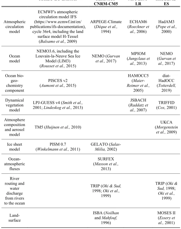
Considering the selected simulations for this study, four different GCMs provided the necessary initial and boundary conditions. The main components of the GCMs are summarized in Table 2, and their main characteristics can be briefly summarized as follows:

• The ICHEC-EC-EARTH model (http://www.ec-earth.org/) is developed as a part of a European consortium. This model is based on the seasonal forecasting system of ECMWF. It can be used as a classical climate model and as an Earth System Model also (by adding atmospheric chemistry, aerosols, ocean bio-geo-chemistry, dynamic vegetation, and Greenland ice sheet).

• CNRM-CERFACS-CNRM-CM5 is an Earth System Model (Voldoire et al., 2013), which is based on the coupling of several models. It is a developed version of the CNRM-CM3, which can reproduce well the large- scale circulation, the Asian monsoon, and the Arctic sea ice cover.

However, it also has some deficiencies, e.g., underestimation of the tropical sea surface temperature, overestimation of precipitation, or weak southern ocean circulation. The model’s horizontal resolution is 1.4° in the atmosphere and 1° in the ocean.

• MPI-M-MPI-ESM-LR (Giorgetta et al., 2013) is based on the coupled GCMs, namely, the ECHAM6 atmospheric submodel and the MPIOM ocean submodel. Other subsystem models (for land and vegetation as well as marine geochemistry) are also included in MPI-M-MPI-ESM-LR.

• HadGEM2-ES is an Earth System Model (Collins et al., 2011), developed from the HadGEM1. The atmospheric component has 38 vertical layers, and it has a horizontal resolution of 1.25° × 1.875° in latitude and longitude, respectively. A large-scale hydrology module has also been introduced into HadGEM2. Considering aerosols, eight species are available in HadGEM2, from which nitrate (only if tropospheric chemistry is used), fossil-fuel organic carbon, and biogenic aerosols are new.

Table 2. The applied submodels in the GCMs used in this study ICHEC-EC-EARTH

CNRM- CERFACS- CNRM-CM5

MPI-M- MPI-ESM-

LR

MOHC- HadGEM2-

ES

Atmospheric circulation

model

ECMWF's atmospheric circulation model IFS (https://www.ecmwf.int/en/

publications/ifs-documentation), cycle 36r4, including the land

surface model H-Tessel (Balsamo et al., 2009)

ARPEGE-Climate (Déque et al.,

1994)

ECHAM6 (Roeckner et

al., 2006)

HadAM3 (Pope et al.,

2000)

Ocean model

NEMO3.6, including the Louvain-la-Neuve Sea Ice

Model (LIM3) (Rousset et al., 2015)

NEMO (Gurvan et al., 2017)

MPIOM (Jungclaus et

al., 2013)

NEMO (Gurvan et

al., 2017) Ocean bio-

geo- chemistry component

PISCES v2 (Aumont et al., 2015)

HAMOCC5 (Maier- Reimer et al.,

2005)

diat- HadOCC (Totterdell,

2019) Dynamical

vegetation model

LPJ-GUESS v4 (Smith et al., 2001; Lindeskog et al., 2013)

JSBACH (Raddatz et

al., 2007)

TRIFFID (Cox, 2001) Atmosphere

composition and aerosol

model

TM5 (Huijnen et al., 2010) UKCA

(Morgenstein et al., 2009) Ice sheet

model

PISM 0.7

(Winkelmann et al., 2011)

GELATO (Salas- Mélia, 2002) Ocean-

atmospheric fluxes

SURFEX (Masson et al.,

2013) River

routing and water discharge from rivers to the ocean

TRIP (Oki & Sud, 1998; Oki et al.,

1999)

TRIP (Oki &

Sud, 1998;

Oki et al., 1999)

Land- surface

ISBA (Noilhan and Mahfouf,

1996)

MOSES II (Essery et al., 2001)

For the current study, the following five RCMs were selected from the 23 different RCMs used in EURO-CORDEX. In the next lines we give a short overview about them.

• The RCA4 model (Kupiainen et al., 2014) was developed from RCA3 (Samuelsson et al., 2011). One of the main important developments is that the former overestimation of soil-heat transfer was reduced by the inclusion of soil carbon. Furthermore, the Kain-Fritsch convection scheme (Kain, 2004) has been updated, so the model distinguishes the shallow and deep convection processes.

• The RACMO22E model is built on the ECMWF physics package merging into the dynamical kernel of HIRLAM (Undén et al., 2002). The model takes into account more soil layers, and it includes a surface runoff scheme.

The leaf area index (LAI) also plays an important role, especially in the surface energy budget. The model applies parametric formulations to treat the ice surfaces (van Meijgaard et al., 2008).

• The REMO model was developed from the Europa-Model (EM) numerical weather prognostic model by adding dynamical core and physics. It uses a terrain-following hybrid coordinate system. The vertical structure encompasses 20 levels, as in the case of EM model. The vertical fluxes are treated implicitly (Jacob and Podzun, 1997).

• The CCLM4-8-17 model is based on the non-hydrostatic Local Model (LM) developed by the German Meteorological Service. The model uses direct coupled components, such as TERRA (surface and soil model) or Flake (fresh-water lake model); whereas ART modul is used for representing chemistry and aerosols (Schättler et al., 2019).

• The ALADIN limited area model was developed from the ARPEGE GCM and the ECMWF Integrated Forecasting System (IFS). The ALARO physics parameterization package, which is suitable to run at convection- permitting fine resolution, was coupled to the ALADIN model (www.euro- cordex.be/meteo/view/en/29038078-ALARO-0+model.html). ALARO uses the Modular Multiscale Microphysics and Transport (MMMT) microphysics scheme that improves the representation of convective precipitation for Europe as validation analysis showed (Giot et al., 2016).

Our study primarily focuses on the plain areas in Hungary and Serbia. Hence, we defined five subregions within the analyzed domain (Fig. 1). Three of them (NHU, CHU, SHU) are located mainly in Hungary, representing the north-central- south regions; the other two (NSR, SSR) are in the northern parts of Serbia (Table 3). Each subregion contains 70 grid cells, covering about ~7800 km².

Fig. 1. Topography map of the target area. The selected subregions are indicated by boxes and their abbreviations.

Table 3. List of the five subregions, which are analyzed in the present study, indicating their abbreviations and geographical coordinates

Region Northern latitude Eastern longitude

NHU (Northern Hungarian Plain) 47.6°‒48.2° 21.5°‒22.4°

CHU (Central Hungarian Plain) 46.8°‒47.4° 20.2°‒21.1°

SHU (Southern Hungarian Plain) 46.3°‒46.9° 19.1°‒20.0°

NSR (Northern Serbian Plain) 45.2°‒45.8° 19.6°‒20.5°

SSR (Southern Serbian Plain) 44.2°‒44.8° 20.5°‒21.4°

Two meteorological variables, namely, daily mean temperature and daily precipitation total are investigated in this study. The analysis focuses on three time periods: the historical time period (1971‒2000), the middle of the 21st century (2021‒2050), and the end of the 21st century (2069‒2098, since some of the RCM simulations do not include the last two years, 2099 and 2100, due to the lack of driving GCM data; however, this selected period can be considered as representing 2071–2100 since a couple of years’ shift does not change the climate change signal on a century scale). The projected changes are calculated

for these three 30-year time slices, for all the five subregions in the case of all RCP scenarios using all RCM simulations selected for this study, hence, a comprehensive comparison analysis is completed.

From the agricultural point of view, the projection of drought conditions is especially important in the plain areas. Therefore, the rainfall variability index (RVI; Gocic and Trajkovic, 2013) is also calculated in this study beside the changes of monthly mean temperature values and the relative changes of monthly precipitation totals. RVI is calculated by the following formula:

ܴܸܫ =^௉೔ି௉_௦ ^ೌ ,

where i is the index of the year, P is the annual precipitation total, Pa is the average annual precipitation total, and s is the standard deviation of annual precipitation totals in the 1971‒2000 reference period.

3. Results and discussion

3.1. Validation (historical experiments versus reference data)

First of all, validation results are analyzed using Taylor-diagrams (Taylor, 2001), for which monthly mean precipitation totals and monthly mean temperature values were calculated for the five subregions, based on the CARPATCLIM datasets as well as all the 10 historical RCM simulations individually. Thus, the reproduction of the mean annual cycle in the RCM simulations can be evaluated against the CARPATCLIM data for the time period 1971–2000.

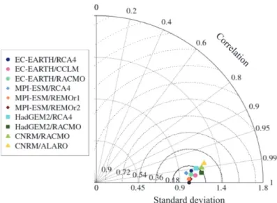
In the case of temperature, no substantial differences can be recognized between the subregions, so only one example is presented here, namely, the CHU subregion (Fig. 2). We can conclude that all the RCM simulations perform well, as the correlation coefficient is above 0.95 in every case, and all the symbols, indicating the individual RCM simulations, are close to the reference black point, which represents CARPATCLIM data. A small difference occurs in relation with the driving GCM: the two least well-performing RCM simulations were both driven by the CNRM-CERFACS-CNRM-CM5 (indicated by triangles in Fig. 2). It can also be seen that the driving GCM of the best overall performing RCM simulations was the MPI-M-MPI-ESM-LR (indicated by diamonds in Fig. 2).

Fig. 2. Taylor-diagram for the CHU subregion, based on temperature data (1971‒2000).

Different driving GCMs are marked with different symbols; each simulation is indicated by a unique color. The black point indicates the reference (CARPATCLIM).

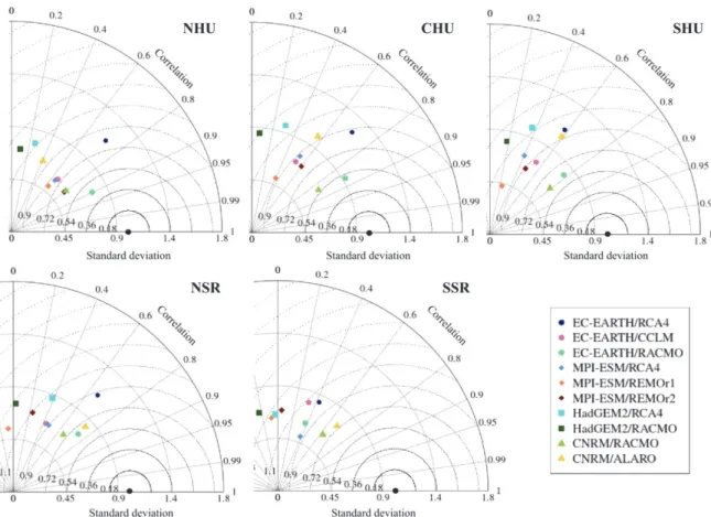
Considering precipitation, validation results show a less successful reproduction of the mean annual cycle compared to temperature. Results are somewhat better in the Hungarian subregions than in the Serbian subregions, where correlation coefficients are generally closer to zero or even negative (Fig. 3) implying very different simulated annual cycle compared to the reference. In spite of that, the CNRM-CERFACS-CNRM-CM5 driven RCM simulations are the least successful in reproducing the reference temperature cycle, this GCM provides the necessary initial and boundary conditions to the overall best performing RCM simulation (CNRM/RACMO) in the case of precipitation. This validation result supports the finding that one cannot choose solely a specific model, which can be considered as the best model from all possible aspects (e.g., Jacob et al., 2007; Torma, 2019). For example, one model is good in the simulation of temperature values, while another model performs more reliably the annual cycle of precipitation, and a third one is capable to simulate extreme values better. In the present case, the effects of different GCMs cannot be separated clearly, as their performances are different considering the different subregions.

Fig. 3. Taylor-diagrams for the five subregions (NHU, CHU, SHU, NSR, SSR) based on precipitation data (1971‒2000). Different driving GCMs are marked with different symbols;

each simulation is indicated by a unique color. The black point indicates the reference (CARPATCLIM).

Kotlarski et al. (2014) discussed a validation analysis of the CORDEX simulations (Giorgi et al., 2009) with the ERA-Interim driving data using the E- OBS database (Haylock et al., 2008) as a reference. Overall temperature biases were found to be smaller than 1.5 °C for the European continent, but in the case of precipitation, larger (~ 40%) over- and underestimations can be seen. Torma (2019) validated the EURO-CORDEX and MED-CORDEX projections for the 1989‒2008 time period using altogether nine ERA-Interim driven RCM simulations. This study found that temperature bias is between ‒3 °C and +3 °C in the Pannonian region. In the case of precipitation, the RCM-ensemble could reproduce the annual cycle quite well in general, but with a more dominant maximum in June.

For the validation of RVI, the CARPATCLIM database served as a reference. The best agreement can be found in the SSR subregion, where there were 15 dry years according to the CARPATCLIM, and all the RCMs simulated the number of dry years between 13 and 17 (i.e., ±2 years compared to the reference). The least agreement can be found in the NHU and SHU subregions, where four RCMs simulated more or less dry years by at least 3 years compared to the reference.

3.2. The projected temperature and precipitation changes

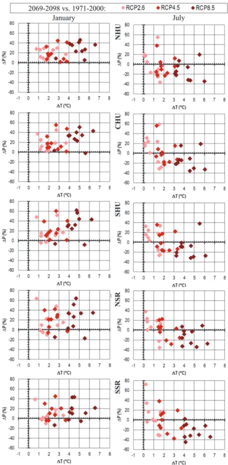
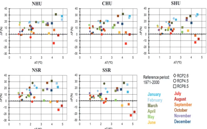
Since the two most important climatic variables are temperature and precipitation in terms of the agricultural activities being dominantly present in the target regions, we continue the analysis with the projected monthly mean temperature and precipitation changes for the five subregions taking into account the three different RCP scenarios. The climatic variables were analyzed together by evaluating the two-dimensional or bi-variate changes of the spatial averages of the subregions (temperature changes are represented horizontally, whereas precipitation changes appear vertically). In Fig. 4, two selected months are shown, namely, January and July (because in the present climate, these are the coldest and the warmest months of the year, respectively). The diagrams summarize the predicted changes by the end of the 21st century on the basis of the 10 individual RCM simulations. Results showing average bi-variate changes reflect the uncertainty of projections due to the model physics. It can be clearly seen that higher temperature values are very likely to occur in the future.

January (and overall the winter half year) will be wetter, especially in the northern subregions, whereas July (and August) will tend to become drier, especially in the case of RCP8.5. The projected temperature changes for RCP2.6 and RCP4.5 are closer to each other, while RCP8.5 induces the greatest regional warming. This can be explained by the definition of the RCP scenarios themselves: i.e., RCP8.5 indicates a radiative forcing change of 8.5 W/m² by the end of the 21st century compared to the pre-industrial era (whereas RCP2.6 and RCP4.5 assumes only a change of 2.6 W/m² and 4.5 W/m², respectively). Since temperature is highly correlated with radiation, the conclusion is straightforward: the largest increase is projected in the case of RCP8.5. The smaller overall difference between the other two scenarios can be expected, because the difference between the assumed radiative forcing changes is smaller between RCP2.6 and RCP4.5 than either between RCP2.6 and RCP8.5, or between RCP4.5 and RCP8.5.

In the case of RCP2.6, the smallest multi-model average temperature increase in January (1.88 °C) is projected for SHU (where the entire range from all the 10 RCM simulations is 0.82‒3.41 °C), and the largest average warming (1.92 °C) is only slightly greater than the smallest, and is predicted for the neighboring subregions: NSR (where the entire range considering all the 10 RCM simulations is 0.80‒3.41 °C, quite similar to SHU) and CHU (where the entire range considering all the 10 RCM simulations is 0.91‒3.68 °C, shifted slightly by 0.1‒0.2 °C relative to NSR and SHU). Smaller overall warming is projected for July, the projected temperature change is ~ 1 °C; the entire range considering all the 10 RCM simulations and the five subregions is 0.07‒1.74 °C implying a smaller variability of simulation results compared to January.

Partially due to the small variability and average values, the difference between the subregions is quite small.

Fig. 4. Projected changes of precipitation (y-axis) and temperature (x-axis) in the five subregions according to the three RCP scenarios (represented by different colors) for the 2069‒2098 time period in January (left column) and July (right column) based on the 10 RCM simulations. The reference period is 1971‒2000.

Taking into account the RCP4.5 scenario, the projected change based on the multi-model mean for January is more than +2.5 °C in all the five subregions; the greatest change on average (2.71 °C) is likely to occur in the northernmost subregion, NHU (where the entire range considering all the 10 RCM simulations is 1.79‒3.82 °C). For July, an increase by ~ 2 °C on average is projected, with the largest change on average (2.28 °C) for the southernmost subregion, SSR (where the entire range considering all the 10 RCM simulations is 1.55‒3.74 °C). According to the RCP8.5 scenario, temperature values in January will be higher on average by at least 4.5 °C (in NHU it is 4.9 °C on average and the entire range considering all the 10 RCM simulations is 2.73‒6.61 °C) compared to the historical time period. In the case of July, the smallest change on average (4.15 °C) is projected for the northernmost subregion, NHU (where the entire range considering all the 10 RCM simulations is 3.11‒6.03 °C) and the greatest on average (4.83 °C) for the southernmost subregion, SSR (where the entire range considering all the 10 RCM simulations is 4.00‒6.59 °C). The projected monthly mean warming for the mid- and late- century is compared in Fig. 5 (since the differences between the subregions are small in projected temperature changes, diagrams show the overall spatial averages), thus the different regional warming trends of the three scenarios can be evaluated for all months. RCP8.5 induces continuous warming in all months;

most RCM simulations (at least 7 RCMs from the 10 RCMs in each month) project even accelerating regional warming in the plain areas of Hungary and Serbia. All the 10 RCM simulations predict such an increasing rate of warming in May, July, August, and September. Contrary to this, the projected monthly mean regional warming tends to slow down during the second half of the 21st century in the case of the RCP4.5 scenario; all the 10 RCM simulations project less warming between the middle and late 21st century in January, July, and August than the estimated warming between the end of the 20th century and the middle of the 21st century. However, an accelerating temperature increase is projected for April, May, and November by at least half of the RCM simulations. Moreover, many RCM simulations projects temperature decrease during the second half of the 21st century in the case of the RCP2.6 scenario;

more specifically, at least half of the RCM simulations predicts such changes for May, July, August, October, and November (the number of RCM simulations with projected cooling during this coming 50 years is 7, 8, 5, 6, and 6, respectively).

Fig. 5. Projected monthly mean temperature changes averaged for the 5 subregions (ΔT) using the three RCP scenarios (represented by different colors) for the 2069‒2098 and 2021–

2050 time periods based on the 10 RCM simulations. The reference period is 1971‒2000.

The projected mean precipitation changes show substantially higher variability than temperature projections. January (which is currently one of the driest months in the region) is very likely to become wetter, especially in the northern subregions (i.e., NHU and CHU), where all of the 10 RCM simulations

RCP2.6 RCP4.5 RCP8.5

Linear warming rate Warming in mid-century = warming in late-century

0 1 2 3 4 5 6 7

-1 0 1 2 3 4 5 6 7

∆T by late-century (°C)

∆T by mid-century (°C)

December

0 0

1 2 3 4 5 6 7

-1 0 1 2 3 4 5 6 7

∆T by late-century (°C)

∆T by mid-century (°C)

January

0 0

1 2 3 4 5 6 7

-1 0 1 2 3 4 5 6 7

∆T by late-century (°C)

∆T by mid-century (°C)

February

0

0 1 2 3 4 5 6 7

-1 0 1 2 3 4 5 6 7

∆T by late-century (°C)

∆T by mid-century (°C)

March

0 0

1 2 3 4 5 6 7

-1 0 1 2 3 4 5 6 7

∆T by late-century (°C)

∆T by mid-century (°C)

April

0 0

1 2 3 4 5 6 7

-1 0 1 2 3 4 5 6 7

∆T by late-century (°C)

∆T by mid-century (°C)

May

0

0 1 2 3 4 5 6 7

-1 0 1 2 3 4 5 6 7

∆T by late-century (°C)

∆T by mid-century (°C)

June

0 0

1 2 3 4 5 6 7

-1 0 1 2 3 4 5 6 7

∆T by late-century (°C)

∆T by mid-century (°C)

July

0 0

1 2 3 4 5 6 7

-1 0 1 2 3 4 5 6 7

∆T by late-century (°C)

∆T by mid-century (°C)

August

0

0 1 2 3 4 5 6 7

-1 0 1 2 3 4 5 6 7

∆T by late-century (°C)

∆T by mid-century (°C)

September

0 0

1 2 3 4 5 6 7

-1 0 1 2 3 4 5 6 7

∆T by late-century (°C)

∆T by mid-century (°C)

October

0 0

1 2 3 4 5 6 7

-1 0 1 2 3 4 5 6 7

∆T by late-century (°C)

∆T by mid-century (°C)

November

0

project increased precipitation by the end of the 21st century compared to the reference period. However, some simulations project decreasing precipitation monthly totals in the southern subregions, especially when the RCP8.5 scenario is taken into account (e.g., the projected mean change in January is 22% on average in NSR, and the entire range is between ‒17% and 64%). On the contrary, a general decreasing trend is likely to occur in July according to the most RCM simulations (except for the case of RCP2.6), but the uncertainty of projections is quite high due to different parameterizations in RCMs. More specifically, RACMO simulations (driven by either the HadGEM2, CNRM, or EC-EARTH models) predict opposite, greater positive changes in July precipitation for RCP4.5 and RCP2.6, whereas the projections of precipitation for RCP8.5 imply either much less, or even negative changes by the end of the 21st century. Overall, we can conclude that the greater the assumed radiative forcing change and the more southern the subregion is located, the more pronounced the drying trend will be in July. So the greatest multi-model mean monthly precipitation decrease (‒22%) is projected in the case of RCP8.5 for SSR (where the entire range considering all the 10 RCM simulations is between

‒45% and 2%).

Fig. 6 shows the projected multi-model mean temperature and precipitation changes by 2069‒2098 for all the 12 months for the five subregions, taking into account the three RCP scenarios. As we already mentioned above, the differences between RCP2.6 (indicated by diamonds) and RCP4.5 (indicated by circles) is relatively small, about 1 °C, while RCP8.5 (indicated by squares) can be distinguished more clearly from the other two scenarios (the difference between RCP4.5 and RCP8.5 is about 2–3 °C). Considering temperature, solely increasing trend occurs for all the monthly averages. The greatest increase, 5.16 °C, is projected for August in SSR – this is the only case when the projected multi-model mean change exceeds 5 °C. Furthermore, the projected regional warming exceeds 4 °C in January, February, July, August, and September in all the five subregions in the case of RCP8.5. Similarly, greater warming can be expected in mid- and late-summer, early-autumn, and mid- and late-winter in the case of RCP4.5, while in the case of RCP2.6, the intra-annual variation of the monthly mean projected warming values is substantially smaller.

Fig. 6. Projected changes of precipitation (y-axis) and temperature (x-axis) in the five subregions according to the three RCP scenarios (represented by different symbols) for the 2069‒2098 time period in the 12 months (different colors) based on the multi-model mean of 10 RCM simulations. The reference period is 1971‒2000.

Considering precipitation, Fig. 6 shows that most of the months will likely become wetter by the end of the 21st century compared to the reference period according to the multi-model average of the 10 RCM simulations. The greatest increase (> 20%) is projected for January, February, and March in all the 5 subregions in the case of all the RCP scenarios. Also, quite high increase (> 15%) is projected in the subregions for December, November, October, and April (except for SHU). Overall, the greatest multi-model mean precipitation change (+32%) is projected for CHU for March, in the case of RCP8.5. Drier conditions are projected only for summer and early autumn, however, different scenarios imply different overall results. A clear drying trend can be seen in July (between ‒13 and ‒22%) and August (up to ‒17% in SSR) in the case of RCP8.5, i.e., assuming high radiative forcing change. Drier conditions are likely to occur in the southern regions even in June (the projected precipitation change is ‒1% in NSR and ‒7% in SSR) and in September (the projected precipitation change is ‒2% in SHU, –1% in NSR, and ‒5% in SSR). If RCP4.5 scenario is taken into account the multi-model mean precipitation is projected to decrease only in July in most subregions, the greatest change is projected for NHU (–4%)

and SSR (–3%); however, the predicted mean drying trend is substantially less than in the case of RCP8.5 due to the smaller projected decreases of the individual RCM simulations for RCP4.5. In the case of the RCP2.6 scenario, none of the months can be expected to become substantially drier in the future.

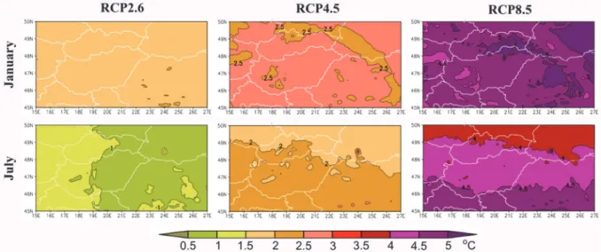
The spatial distribution of the multi-model mean projected temperature changes by the end of the 21st century is presented in Fig. 7 for January and July for the three RCP scenarios. As it can already be seen from the results of Figs. 4–6, the greater radiative forcing change results in higher temperature-increase regionally as well as globally (IPCC, 2013), which is quite evident from the definition of the RCP scenarios. The patterns of the projected changes reflect dominantly the topography of the domain in January, while a clear zonal structure can be seen in the maps of multi-model mean warming for July, especially for RCP4.5 and RCP8.5. In January, somewhat smaller temperature increase (< 3 °C) is projected for the Carpathian Mountains compared to the plain areas in the case of RCP4.5, while it is the opposite in the case of RCP8.5, namely, the highest projected increase (> 5 °C) appears in the mountainous regions. In July, an east- west difference will emerge in the case of RCP2.6, with slightly higher values in the western parts of the domain. The patterns are different in the case of RCP4.5 and RCP8.5, namely, a north-south gradient appears with greater mean increase (> 2 °C and > 4.5 °C, respectively) in the southern regions. The zonal gradient is the highest for RCP8.5 when the overall warming is also greater.

Fig. 7. Projected changes of temperature according to the three RCP scenarios for 2069‒2098 relative to 1971‒2000 in January and July based on the multi-model mean of 10 RCM simulations.

As a consequence of these projected monthly mean temperature increases, temperature-related extremes are expected to change. Specifically, warm extremes (e.g., tropical nights with daily minimum temperature exceeding 20 °C) will occur more frequently and with a longer duration in the future, whereas cold extremes (e.g., frost days with daily minimum temperature below 0 °C) are very likely to decrease by the late-century. The Pannonian Basin is analyzed from this aspect by Pieczka et al. (2018), using one specific RCM taking into account RCP4.5 and RCP8.5.

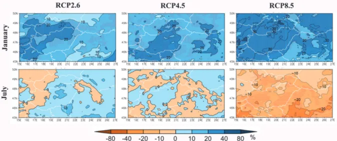
Considering the spatial distribution of precipitation in January and July for the late-century, we can conclude that the greatest changes are projected in the case of RCP8.5, and the differences between RCP2.6 and RCP4.5 are smaller (Fig. 8). In January, multi-model mean precipitation increase exceeding 20% is projected only for the western and northern parts of the domain in the case of RCP2.6. The overall pattern is different from this in the case of RCP4.5, since at least 20% increase is estimated for almost the whole territory of Hungary and the eastern Carpathians. Finally, when taking into account the RCP8.5 scenario, an increasing trend by 20‒30% is likely to occur over most parts of the domain (except the northeastern and southern Carpathians); the projected change is positive according to at least seven RCM simulations in almost the entire domain. Contrary to this, a precipitation decrease is projected for July; this drying trend is more pronounced in the southern part of the domain (i.e., the predicted decrease can exceed 20%). The uncertainty originating from the different RCM simulations is higher, which is indicated by the hatched areas covering overall less part of the domain in July than in January. The multi- model mean of July precipitation change is much smaller for either RCP2.6 or RCP4.5 than for RCP8.5, which is due to the fact that RCM simulations result in increasing and decreasing precipitation trends more diversely, thus they eliminate each other.

Since the greatest temperature and precipitation changes are projected by the end of the 21st century for the RCP8.5 scenario, a more detailed analysis based on the multi-model mean of the 10 RCM simulations is presented in Figs.

9‒12 for each month grouped by season. In the case of temperature, all the RCMs simulate a clear increasing trend, i.e., only positive changes by the late- century compared to the reference period. However, precipitation projections show higher variability within the ensemble of RCM simulations, including even different signs of changes (therefore, hatching on the precipitation maps indicates where at least seven model-simulations agree in the sign of the projected change with the change exceeding ±10%).

Fig. 8. Projected changes of precipitation according to the three RCP scenarios for 2069‒2098 relative to 1971‒2000 in January and July based on the multi-model mean of 10 RCM simulations. Hatched areas show where at least seven simulations indicated the same direction of change, and the projected change was at least ±10%.

In summer, the multi-model mean warming is the most pronounced in August, when the projected change can exceed 5 °C in the southern parts of the domain (Fig. 9). Similar zonal pattern appears in July, the difference between August and July is about 0.5 °C. The overall smallest temperature increase is predicted for June, but a mean change of at least 3 °C is predicted even in the northwesternmost parts of the domain (where the smallest increase appears).

Considering precipitation, Fig. 8 already shows the multi-model mean decreasing trend projected for July, which can be larger than ‒20% in the southern parts of the domain. August is projected to become also drier, however, the multi-model mean change is closer to zero compared to July, and the precipitation decrease is more robust in the southeastern part of the domain.

Contrary to these, a clear north-south difference can be recognized in June, i.e., there is an increasing trend in Austria, Slovakia, Ukraine, and Hungary, whereas decreasing trend in Slovenia, Croatia, Serbia, and the most parts of Romania;

note that the uncertainty is quite high, as the multi-model mean precipitation change is within the range of (–10%; 10%) with very few hatched areas (only outside the Pannonian Basin in the plain areas south and east from the Carpathian mountain ranges).

Fig. 9. Projected changes of temperature and precipitation according to the RCP8.5 scenario for 2069‒2098 relative to 1971‒2000 in the summer months based on the multi-model mean of 10 RCM simulations. In the case of precipitation, hatched areas show where at least seven models indicated the same direction of change, and the projected change was at least ±10%.

Topography-dependent warming is projected in winter (especially in January and February), the projected multi-model mean temperature change by the end of the 21st century is 4‒5.5 °C (3.5–4.5 °C in December) compared to the reference period (Fig. 10). The greatest increase (> 5 °C) is projected in the Carpathians, except for December, when somewhat smaller (> 4 °C) increase is projected for the eastern parts of Hungary and Transylvania. In the case of winter precipitation, the projected multi-model mean monthly changes imply wetter conditions, moreover, most of the RCM simulations agree on the sign of the predicted change in all the three winter months. The smallest change is projected for December; in January and February the simulated change is at least 20% almost in the entire domain. Considering both meteorological variables simultaneously, one can

conclude that more precipitation is likely to occur in the future in winter, but the rate of snow will be less due to the projected temperature-rise resulting in important consequences from hydrological point of view (e.g., Kis et al., 2017b).

Fig. 10. Projected changes of temperature and precipitation according to the RCP8.5 scenario for 2069‒2098 relative to 1971‒2000 in the winter months based on the multi-model mean of 10 RCM simulations. In the case of precipitation, hatched areas show where at least seven models indicated the same direction of change, and the projected change was at least ±10%.

September is similar to the summer months: the multi-model mean temperature increase shows a zonal pattern (with a warming of 3.5–4.5 °C) together with an overall drying trend projected over the southern and mountainous parts of the domain (Fig. 11). The simulated changes for October and November are more

similar to the projected changes for winter, as an overall 10‒30% precipitation increase is likely to occur (somewhat smaller change is projected for November than for October), the estimated temperature increase is somewhat smaller (< 4 °C) than for winter. Furthermore, the spatial variability within the domain is much smaller than in the winter months.

Fig. 11. Projected changes of temperature and precipitation according to the RCP8.5 scenario for 2069‒2098 relative to 1971‒2000 in the autumn months based on the multi-model mean of 10 RCM simulations. In the case of precipitation, hatched areas show where at least seven models indicated the same direction of change, and the projected change was at least ±10%.

The projected multi-model mean temperature changes for March, April, and May are similar to January and February considering the spatial pattern (i.e., reflecting the topography of the domain), but the predicted values of spring warming are not so high as in winter (Fig. 12). Precipitation is likely to increase

in spring, especially in March (by ~ 30%±10%) with a high agreement in the sign of projected changes. Positive changes are projected by fewer RCM simulations in April, and even fewer in May, thus the multi-model projected change of monthly mean precipitation is smaller in April, and even smaller in May compared to March. The multi-model mean precipitation change even shows a slight decrease in May at the southern border of the domain, since some RCM simulations project drier conditions for the late-century compared to the reference period, especially in the southern part of the domain.

Fig. 12. Projected changes of temperature and precipitation according to the RCP8.5 scenario for 2069‒2098 relative to 1971‒2000 in the spring months based on the multi-model mean of 10 RCM simulations. In the case of precipitation, hatched areas show where at least seven models indicated the same direction of change, and the projected change was at least ±10%.

On the basis of maps with multi-model mean changes, similar changes are projected for the mid-century as for the late-century, but the temperature increase is more moderate (1‒2 °C) and more homogeneous in space. In the case of precipitation, an increase is projected for 2021–2050, except for July and August, when decreasing trend is likely to occur, but with greater uncertainty and smaller overall changes compared to the changes simulated for the 2069‒2098 time period.

In order to analyze the variability of precipitation changes in more details, Fig. 13 shows each simulated monthly precipitation total in January and July during the 30-year period at the end of the 21st century compared to the average monthly total in the 1971‒2000 reference period. Results for the five investigated subregions are quite similar to each other. Therefore, we only present one example here, namely, the SHU subregion (located in the middle among the five subregions regarding the north-south extension). In order to illustrate uncertainty not only due to the climatic variability but also due to the model physics and parameterizations, all the 10 RCM simulations are presented (x-axis) in the diagrams taking into account the three different RCP scenarios (indicated by different colors). The differences between the RCP scenarios are not substantial, which can be explained by the fact that in the case of precipitation, the role of the scenario is relatively low within the full uncertainty range of simulations compared to the choice of the model or to the internal variability (Hawkins and Sutton, 2011). Overall, it can be concluded that greater inter-annual differences occur between the individual monthly anomalies in July in some RCM simulations (e.g., the spread is especially wide in the case of RCM simulations where EC-EARTH or HadGEM2 provide driving inputs to the regional scale), because extremely high precipitation is simulated in a few years.

In the case of RCP8.5, according to four RCM simulations, more than 20 years out of 30 will be drier in July compared to the reference period. In SSR, which is the southernmost subregions among the five analyzed subregions, the same conclusion can be made, but the number of these RCM simulations is six, implying higher confidence in expecting drier Julies in the future. Three RCMs simulated drier July conditions relative to the reference period for all the five subregions at least 20 years out of 30 in the case of RCP8.5 (whereas only one RCM simulated similarly for RCP2.6). When taking into account RCP4.5, none of the RCM simulations resulted in drier Julies with such dominance in all the five subregions, however, unlike other simulations, one RCM simulation (i.e., CNRM_RACMO) projects that at least 20 years out of 30 will be wetter in the future in NHU and CHU (in general, wetter July conditions do not exceed the half of all the 30 years in neither scenario or subregions).

Contrary to July, mainly wetter conditions are simulated for January compared to the reference period; two RCM simulations project more monthly precipitation totals in all the five subregions in at least 20 years out of 30, namely, HadGEM2_RCA4 in the case of RCP4.5 and MPI-ESM_REMOr2 in

the case of RCP8.5. Drier Januaries also occur in the simulations, but less frequently compared to the wetter conditions relative to the reference period in any of the subregions.

Fig. 13. Projected changes of monthly precipitation in January (top) and July (bottom) according to the three RCP scenarios (indicated by different colors) for each year in 2069‒2098 (indicated by crosses) relative to the 1971‒2000 reference period based on the 10 individual RCM simulations (x-axis). Spatial averages for the SHU subregion are shown. The RCM simulations are as follows: (1) CNRM_ALARO, (2) CNRM_RACMO, (3) EC-EARTH_CCLM, (4) EC-EARTH_RACMO, (5) EC-EARTH_RCA4, (6) Had- GEM2_RACMO, (7) HadGEM2_RCA4, (8) MPI-ESM_RCA4, (9) MPI-ESM_REMOr1, (10) MPI-ESM_REMOr2.

Finally, RVI is analyzed as a precipitation-related feature for the entire year, it is calculated for the five subregions. If the RVI value is smaller than zero for a given year that year is considered as a dry year; if the RVI value is less than ‒2, it is considered as an extreme dry year. The projected RVI values for the 2021‒2050 (x-axis) and 2069‒2098 (y-axis) time periods are shown in Fig. 14 based on the 10 RCM simulations, taking into account the three RCP scenarios (indicated by different colors). In order to facilitate the analysis, two lines are drawn in the diagrams at 15 years indicating the half of the entire simulation period. It can be clearly seen that in the future wetter years are likely to occur. This is a quite straightforward consequence of the monthly changes analyzed above, namely, decreasing trend is projected only for July and August, whereas precipitation is likely to increase in the rest and most parts of the year, so overall the annual average total will also increase. The difference between the RCP scenarios is not so remarkable; it may be explained by the role of different sources of uncertainty in the case of precipitation (as the choice of the scenario is not the most important factor discussed by Hawkins and Sutton (2011)).

The number of extreme dry years is obviously smaller than the number of dry years, and their distributions show a closer pattern in the diagrams. In the case of the number of dry years, higher variability can be seen: in some RCM simulations the number of years is close to 15 (which is the half of the investigated time period), while in others, only 5 dry years out of 30 are projected to occur in the future. Extreme dry conditions will tend to occur in 2–

12 years overall during 30-year future time periods in the northern plain subregions (NHU, CHU, SHU), whereas more frequent extreme dry years are likely to occur in the southern subregions (i.e., NSR, SSR). The RVI results for the mid- and late-century are not substantially different implying only very slight changes between these future periods.

Fig. 14. Projected number of dry and extreme dry years based on RVI 2021‒2050 (x-axis) and 2069‒2098 (y-axis) in the five subregions according to the three RCP scenarios (indicated by different colors) based on the 10 RCM simulations (indicated by diamonds).

4. Conclusions

The projected temperature and precipitation changes are analyzed for the Pannonian Basin, focusing on five subregions: the plain areas of Serbia and Hungary in a north-south sequence. For the investigation, 10 RCM simulations are used considering three different RCP scenarios, namely, the RCP2.6, RCP4.5 and RCP8.5. Three time periods were analyzed, one historical (1971‒2000) and two future time periods (2021‒2050, 2069‒2098). Since the greater changes are likely to occur by the end of the 21st century, this time period is presented and discussed in more details in this paper.

On the basis of the results shown here, it can be concluded that higher temperature values can be expected in the plain areas of Serbia and Hungary (and in the whole Pannonian Basin) in the future. The projected change by the end of the 21st century is at least 3 °C in every month. Considering the spatial pattern, zonal structure can be clearly recognized in summer, with greater increase (> 4.5 °C) in the southern parts of the domain; while topography plays the key role in winter, with higher values in the mountainous areas. The higher the assumed radiative change in the scenario, the higher the simulated temperature change, which is due to the strong relationship between the radiative forcing and temperature.

Considering precipitation, a decrease is likely to occur in July and in August; and also in June and in September in the southern subregions. In the rest of the year, wetter conditions are projected for the end of the 21st century compared to the end of the 20th century; the projected increase of precipitation is ~ 20% when taking into account the RCP8.5 scenario.

To conclude, in general, warmer and wetter climatic conditions are likely to occur in the plain areas of Serbia and Hungary in the future, but the amplitudes of the projected changes depend on the applied RCP scenario. In the case of temperature, the presented results are in good agreement with former analyzes (e.g., Bartholy et al., 2007), however, in the case of precipitation, some differences can be seen, i.e. summer drying in not so evident, as former simulations showed (Bartholy et al., 2007; Pongrácz et al., 2014; Kis et al., 2017a).

The obtained results can serve as key input in further impact studies (e.g., Pokovai et al., 2020) for the Pannonian region, thus, appropriate adaptation strategies can be developed to cope with the future regional climatic changes.

Agriculture, water management and energy sector should take into account these projected changes in long-term planning at regional and national scales.

It is important to note that the projection results for the different RCP scenarios can be clearly distinguished in the case of temperature – as the correlation between the radiative forcing (its change serves as the definition of RCP scenarios) and temperature is quite high –, while in the case of precipitation the differences among RCM results are often greater than those among RCPs. This result is fostered by the conclusion of Hawkins and Sutton

(2011), namely, the selected RCM plays a higher role in the uncertainty of the projected precipitation change compared to the applied emission scenario, furthermore, internal variability also shows greater effect generally than in the case of temperature (von Trentini et al., 2019). Therefore, it is advisable to take into account more RCM simulations for those studies, which aim to help decision making, to cover the entire range of uncertainty. All in all, the further improvements of both GCMs and RCMs are still a key issue in order to use as reliable simulations as possible for getting relevant results in impact studies. For this purpose non-hydrostatic approach (e.g. Sasaki et al., 2008; Lyra et al., 2018) will probably provide a better reproduction of precipitation conditions.

Nevertheless, the main challenge due to the high internal variability of precipitation still remains.

Acknowledgements: Research leading to this paper has been supported by the following sources: the Széchenyi 2020 programme, the European Regional Development Fund and the Hungarian Government via the AgroMo project (grant number: GINOP-2.3.2-15-2016-00028), the Hungarian National Research, Development and Innovation Fund under grants K-129162 and K-120605, the Hungarian Ministry of Human Capacities under the ELTE Excellence Program (grant number: 783- 3/2018/FEKUTSRAT), the Ministry of Education, Science and Technological Development, Republic of Serbia (Grant No. TR37003), and the Bilateral science and technological cooperation program between Serbia and Hungary (Grant No. 451-03-02294/2015-09/10 and TÉT_16-1-2016-0135). This study is a contribution to the PannEx Regional Hydroclimate Project of the World Climate Research Programme (WCRP) Global Energy and Water Exchanges (GEWEX) Project. Furthermore, we acknowledge the CARPATCLIM Database compiled with the support of the European Commission in JRC in 2013.

References

Aumont, O., Ethé, C., Tagliabue, A., Bopp, L., and Gehlen, M., 2015: PISCES-v2: an ocean biogeochemical model for carbon and ecosystem studies. Geosci. Model Dev. 8, 2465‒2513.

https://doi.org/10.5194/gmd-8-2465-2015

Balsamo, G., Viterbo, P., Beljaars, A., van den Hurk, B., Hirschi, M., Betts, A.K. and Scipal, K., 2009:

A revised hydrology for the ECMWF model: Verification from field site to terrestrial water storage and impact in the Integrated Forecast System. J. Hydrometeorol. 10, 623‒643.

https://doi.org/10.1175/2008JHM1068.1

Bartholy, J., Pongrácz, R., and Gelybó, Gy., 2007: Regional climate change expected in Hungary for 2071-2100. Appl. Ecol. Environ. Res. 5, 1‒17. https://doi.org/10.15666/aeer/0501_001017 Bihari, Z., and Szentimrey, T., 2013: CARPATCLIM Deliverable D2.10. Annex 3 – Description of

MASH and MISH algorithms. 100p.

Ceglar, A., Croitoru, A-E., Cuxart, J., Djurdjevic, V., Güttler, I., Ivancan-Picek, B., Jug, D., Lakatos, M., and Weidinger, T., 2018: PannEx: The Pannonian Basin Experiment. Climate Serv. 11, 78‒85. https://doi.org/10.1016/j.cliser.2018.05.002

Collins, W.J., Bellouin, N., Doutriaux-Boucher, M., Gedney, N., Halloran, P., Hinton, T., Hughes, J., Jones, C.D., Joshi, M., Liddicoat, S., Martin, G., O'Connor, F., Rae, J., Senior, C., Sitch, S., Totterdell, I., Wiltshire, A., and Woodward, S., 2011: Development and evaluation of an Earth- system model – HadGEM2. Geosci. Model Develop. Discus. 4, 997–1062.

https://doi.org/10.5194/gmdd-4-997-2011

Cox, P., 2001: Description of the „TRIFFID” Dynamic Global Vegetation Model. Hadley Centre technical note 24.

Dalelane, C., Früh, B., Steger, C., and Walter, A., 2018: A Pragmatic Approach to Build a Reduced Regional Climate Projection Ensembles for Germany Using the EURO-CORDEX 8.5 Ensemble. J.

Appl. Meteorol. Climatol. 57, 477‒491. https://doi.org/10.1175/JAMC-D-17-0141.1