DOI:10.28974/idojaras.2020.2.1
IDŐJÁRÁS
Quarterly Journal of the Hungarian Meteorological Service Vol. 124, No. 2, April – June, 2020, pp. 143–156
Return values of 60-minute extreme rainfall for Hungary
Mónika Lakatos*, Beatrix Izsák, Olivér Szentes, Lilla Hoffmann, Andrea Kircsi, and Zita Bihari
Hungarian Meteorological Service Kitabel P. s 1, H-1024, Budapest, Hungary
*Corresponding Author e-mail: lakatos.m@met.hu (Manuscript received in final form February 27, 2020)
Abstract⎯ The rainfall intensity for various return periods are commonly used for hydrological design. In this study, we focus on rare, short-term, 60-minute precipitation extremes and related return values which are one of the relevant durations in the planning and operating demands of drainage and sewerage systems in Hungary. Time series of 60-minute yearly maxima were analyzed at 96 meteorological stations. To estimate the return values for a given return period, the General Extreme Value (GEV) distribution was fit to the yearly maxima. The GEV fit and also the Gumbel fit (GEV Type I.) were tested. According to the goodness of fit test results, both GEV and Gumbel distributions, are adequate choices. The return values for 2, 4, 5, 10, 20, and 50 year return periods are illustrated on maps, and together with their 95% confidence intervals, are listed in tables for selected stations. The maps of return values demonstrate that the spatial patterns of the return values are similar, although the enhancing effect of orography can be explored in the Transdanubia region and in the North Hungarian Range. As the return period is increasing, so the range of the confidence are widening as it is expected.
Key-words: extreme precipitation, rainfall intensity, GEV, return level
1. Introduction
In recent decades, an increasing number of studies have reported about the presence of significant positive trends in precipitation extremes in Europe (e.g., Alexander et al., 2006; Klein Tank and Konnen, 2003; Moberg et al., 2006; Zolina et al., 2009).
The observed more frequent heavy precipitation events are also consistent with increasing amounts of water vapor in the atmosphere due to global warming (Allen and Ingram, 2002; Willett et al., 2008). The warming climate induces increasing frequency of extreme precipitation in some region. Significant trends in precipitation extremes over Europe have been found since the middle of the 20th
century in earlier regional studies for Northern Europe (Groisman et al., 2005), the UK (Fowler and Kilsby, 2003), the Mediterranean region (Pujol et al., 2007), and western and eastern parts of the Czech Republic (Kysely, 2009) and Poland (Łupikasza et al., 2010). E.J.M. van den Besselaar and co-authors (Besselaar et al, 2013) showed that despite the considerable decadal variability, 5-, 10-, and 20-year events of 1-day and 5-day precipitation amounts for the first 20 years in the period 1951-2010 became more common in the analyzed 60 years for the daily precipitation series from the European Climate Assessment and Dataset (ECA&D, http://www.ecad.eu) project (Klein Tank et al., 2002; Klok and Klein Tank, 2008).
Considering the precipitation changes in Hungary, the decrease of the yearly precipitation sum is not remarkable, it is 3% from 1901 to 2019. From the beginning of the 1990s, precipitation has been increasing both on annual and seasonal scales, however, this rise is not significant. Recent years have been dominated by extremes. The magnitude of the change in precipitation intensity (mm/day) is about 1.3 mm/day in the countrywide average. The number of days with daily sum above 20 mm increased by 1 day in the period 1901-2019.
Estimation of precipitation extremes are essential for the planning of important infrastructure, such as water control systems, reservoirs, dams, and urban runoff. The rainfall intensity for various return periods are commonly used for hydrological design (Hailegeorgis, et al., 2013). The Hungarian Meteorological Service provides climate services on return periods of short-term precipitation (10 min, 20 min, 30 min, 60 min, 180 min) to the authorities responsible for roads, railways, hydrological and urban planning. The return period is the average time between the occurrences of extremes of a specified size. The return period of extremely high values of short-term rainfall has shortened in recent years in Hungary, as it is shown in a case study for the Pécs- Pogány meteorological station (Lakatos and Hoffmann, 2019). Lakatos and Hoffmann (2019) also published the intensity-duration-frequency (IDF) curves for the Pécs-Pogány station. The IDF curves are commonly used in planning to describe the return period associated with a given rainfall event. Earlier studies of the short-term precipitation intensity covered the period 1967–1990, when the rainfall was registered by ombrographs (Váradi and Nemes, 1992). The return values (or design values) for different return period were estimated by Váradi and Nemes for 26 stations in Hungary. Gayer and Ligetvári (2006) refer to results of Váradi and Nemes as an exemplary work in the municipal water management planning in Hungary. High intensity, short-term showers, typically 1 hour or less, occasionally up to 3 hours has the greatest impact on the urban environment (Gayer and Ligetvári, 2006). Due to the recent and projected climate change, existing design criteria for infrastructure should be revised as it is pointed out in Varga et al., 2016.
In this study, we focus on rare, short-term, hourly, namely 60-minute precipitation extremes and related return values which are relevant in the planning and operating demands of drainage and sewerage systems in Hungary.
2. Data
The focus area is Hungary. Automatic weather stations replaced the ombrographs in many places in Hungary, particularly from the late 1990s. As a result of automatization, 22-year-long 10 minutes data series are available to analyze the behavior of the sub-daily precipitation for Hungary from 1998. The 10-minute sums of precipitation are stored in the digital meteorological database of the Hungarian Meteorological Service. The 10-minute data was used to derive all the 60-minute rainfall sums which are used in this study. Then the yearly maxima of the 60-minute rainfall were computed for each station to apply extreme value analysis. Time series of yearly maxima were analyzed at 96 meteorological stations in this paper (Fig. 1). The analysis performed here covers almost the complete automatic weather station network in Hungary.
Stations with lot of missing data and with shorter time series were excluded from this study. Time series of the yearly maxima have been quality controlled, and their temporal homogeneity were checked using the MASH (Szentimrey, 1999) method before applying extreme value analysis. The MASH method is an internationally well-known homogenization procedure, one of the best performing methods according to the benchmarking test executed in the COST (European Cooperation in Science and Technology) Action ES060: advances in homogenization methods of climate series: an integrated approach (HOME) (Venema et al., 2012). Erroneous data and inhomogeneities may severely affect the extremes. Therefore, great care must be taken during the decision making on inclusion or exclusion of the erroneous data, as sometimes it is difficult to distinguish the extremes and outliers.
Fig. 1. Automatic weather stations used in this study. Additional statistics are shown for the labeled stations.
3. Methods
The objective of our analyses is to estimate the amount of rainfall falling at a given point for a fixed duration (60 minutes in our case) and a given return period. To estimate the return values for a given return period, the extreme value theory and relating statistical methods have to be applied. Extremes can be found in the tails of the probability distribution. An introduction to extreme value theory can be found in many publications, for example in Coles (2001) and Katz (2002).
In recent years, two statistical approaches are frequently used in modeling extreme rainfall events: the model of annual maxima (block maxima) and the peaks over threshold (POT) model (Coles, 2001). The most common approach in modeling extremes involves fitting a statistical model to the annual extremes in a time series of data. The classical POT model defines a threshold and considers all events with intensity higher than this threshold. The block maxima are usually modeled by a Gumbel or a generalized extreme value (GEV) distribution (Katz et al., 2002), while the POT is modeled by the generalized Pareto distribution (Katz et al., 2002; Coles, 2001). Despite its advantages, the POT model is much less applied in the analysis of hydrological extremes (Madsen et al., 1997). The World Meteorological Organization (WMO) report entitled “Statistical Distributions for Flood Frequency Analysis” (Cunnane, 1989) provides a review of probability distributions of extreme values and methods for estimation of their parameters. Other WMO source in this topic is the “Guidelines on Analysis of extremes in a changing climate in support of informed decisions for adaptation” (Klein Tank, 2009).
The GEV distribution was introduced by Jenkinson (Jenkinson, 1955). It describes the three types of extreme value distributions for block maxima of any variable (Coles, 2001). The distribution of the block maxima converges to a GEV distribution G(x) while the record length approaches infinity. The three- parameter GEV distribution can be defined in the form
; , , = − 1 + / , (1)
where µ is the location, σ is the scale, and ξ is the shape parameter. Note that σ and 1 + ξ(x-μ)/σ must be greater than zero. Depending on ξ, the G(x) converges to one of three types: Type I (Gumbel) (ξ = 0), Type II (Fréchet) (ξ > 0), and Type III (Weibull) (ξ < 0). Thereby the shape parameter determines whether the fitted distribution will have a finite lower bound, a finite upper bound, or no bound. In the unbounded case, the shape parameter has value zero, and the GEV distribution becomes the well-known Gumbel distribution (Gumbel, 1958), which have been used extensively in hydrology, meteorology, and engineering.
The Gumbel/Type 1 distribution have been applied in hydrology to model floods
and extreme rainfalls (Chow et al., 1988; Stedinger et al., 1993). According to several studies, extreme 24-hour precipitations follow Type II distribution (heavy upper tail; ξ > 0) (Wilks, 1993; Koutsoyiannis and Baloutsos, 2000; Katz et al. 2002; Coles and Pericchi, 2003; Coles et al., 2003; Koutsoyiannis, 2004).
Fréchet distribution represents the lowest risk for technological architecture, as design values are higher than for Type I (Gumbel) and Type III (Weibull).
From the fitted extreme value distribution, we can estimate the return value which is defined as a value that is expected to be equaled or exceeded on average once in every time interval T (return period), with a probability of p= 1/T. Therefore, the return values (z) can be calculated from the Eq.(1) by inverting the GEV distribution in the case of a stationary climate (Matyasovszky, 2002):
. =− ln (− ) +
. = (− + ) (2)
. =− (− ) + .
The POT method was applied by Lakatos and Matyasovszky for 10-minute precipitations measured at Baja meteorological station. Pareto distribution was fitted to 10-minute sums of rainfalls above a specified threshold to estimate the distribution of extreme values (Lakatos and Matyasovszky, 2004).
In accordance with the recent practice of the Hungarian Meteorological Service, the GEV distribution is fitted to the time series of annual maxima/minima. The data are stored in the digital meteorological database, and functions to estimate the different return values are implemented and operated within the digital database. These functions are based on the procedure that was published by Tibor Faragó (Faragó, 1989; Faragó et al., 1989; Faragó and Katz, 1990). The return values pertaining to predefined return periods (2, 4, 5, 10, 20, 50, 100, and 200 years) are computed and displayed for various meteorological elements, e.g., for the short-term precipitation sum (10-, 20-, 30-, 60-, and 180-minute).
In this paper GEV distribution was fit to yearly maximum series of 60- minute rainfall measured at 96 automatic weather stations (AWS) in the period of 1998–2019 first. Moreover, the Gumbel fit was tested. The second step was the computation of the return values for 2, 4, 5, 10, 20, 50 years together with their 95% confidence intervals. Maximum-likelihood method was used to estimate µ location, σ scale, and ξ shape parameters of the GEV distribution (Prescott and Walden, 1980). The distribution fit and the computation of the return values and the 95% confidence intervals were executed by applying the R statistical software (R Core Team, 2012). The return values are illustrated on maps. The results of the distribution fit and the bounds of the confidence intervals are presented in tables for 10 selected meteorological stations.
4. Results and discussion
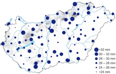
Return value can be interpreted as the value that is expected to be equal or exceeded on average once in every return period (T), or with probability p=1/T in any given year. The T= 2, 4, 5, 10, 20, and 50-year return values of the 60 minutes rainfall can be seen on the maps in Figs. 2-7 for Hungary. The GEV distribution were fitted to the 60-minute yearly maxima at the 96 measuring sites, and the return values were then derived. Return values calculated for return periods frequently used in engineering practice are ccalculated on the maps. For instance, the intensity of a 60-minute event which would be exceeded once every 2 years, on average, is shown in Fig. 2. The maps of return values demonstrate that the longer the return period the greater the pertaining return value. The spatial patterns of the return values are similar on each map. The enhancing effect of orography can be explored in the Transdanubia region and in the North Hungarian Range, although it is not pronounced. It often occurs that hills and mountains enhance the moving air masses, and the largest intensity can be experienced afterwards under the mountains. On the maps greater values appear also in plain regions, typically in the southeast. The reason for this pattern is that short-duration high-intensity rainfalls happen mainly through local convective cells, which have similar physical properties less respective of geographical location. Occasionally, intensive rainstorms evolve during fast moving cold fronts, and sometimes the storms structured in squall-line and cause extreme rainfall in a very short time interval.
Fig. 2. 2-year return values of the 60-minute rainfall.
Fig. 3. 4-year return values of the 60-minute rainfall.
Fig. 4. 5-year return values of the 60-minute rainfall.
Fig. 5. 10-year return values of the 60-minute rainfall.
Fig. 6. 20-year return values of the 60-minute rainfall.
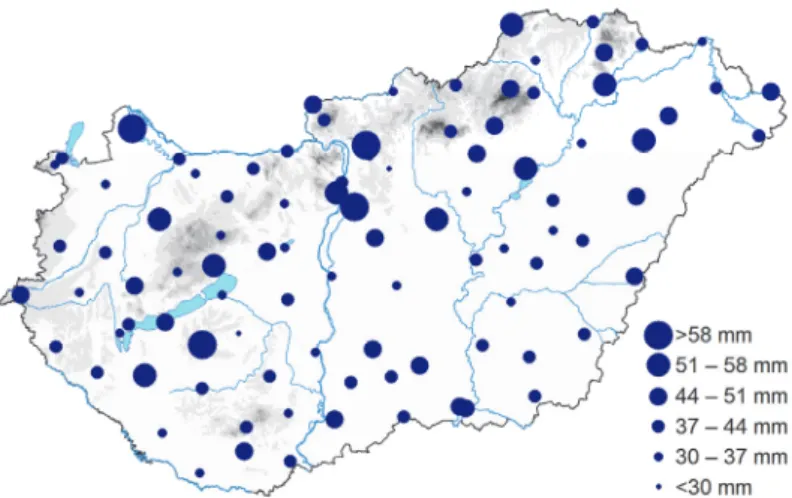
Fig. 7. 50-year return values of the 60-minute rainfall.
Over the years, the GEV distribution has become a widely used model in extreme value analysis. Although it is essential to draw attention to the fact that the GEV distribution is simply a model, our observational series and associated statistics do not precisely follow the theory. The GEV fit procedure resulted in the µ (location), σ (scale), and ξ (shape) parameters of the asymptotic probability distribution function. Depending on the value of the ξ parameter, the extremes will converge to the Gumbel (ξ=0), Fréchet (ξ > 0), or Weibull (ξ < 0) types.
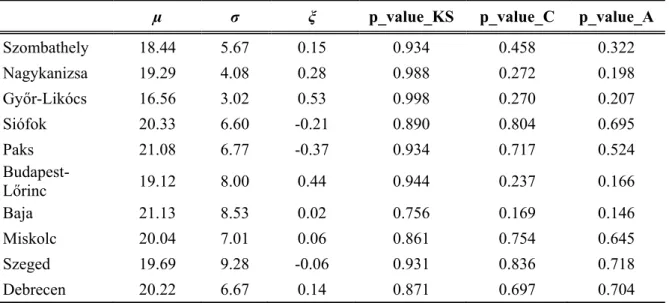
According to our analysis, the ξ parameter is under -0.1, at about one fourth (27%) of the stations resulting the upper bound, and ξ is above 0.1 at 42 % of the stations resulting the lower bound in the extreme value distribution. Table 1 contains these three parameters (µ, σ, ξ) for 10 selected stations from the 96 in total, equally covering the territory of Hungary. Possibly the ξ parameter varies according to the dominating precipitation systems and orographic effects. The
larger positive ξ values appear at stations located chiefly in the western and southern part of Hungary which is under the influence of the Atlantic and Mediterranean climate respectively. The largest ξ value appears at observation stations operating in rural areas of the capital.
Table 1. The µ (location), σ (scale), and ξ (shape) parameters of the GEV distribution and the p-values that are the outputs of the goodness of fit tests for GEV (p_value_KS) and Gumbel (p_value_C and p_value_A) distribution for selected stations
µ σ ξ p_value_KS p_value_C p_value_A
Szombathely 18.44 5.67 0.15 0.934 0.458 0.322
Nagykanizsa 19.29 4.08 0.28 0.988 0.272 0.198
Győr-Likócs 16.56 3.02 0.53 0.998 0.270 0.207
Siófok 20.33 6.60 -0.21 0.890 0.804 0.695
Paks 21.08 6.77 -0.37 0.934 0.717 0.524
Budapest-
Lőrinc 19.12 8.00 0.44 0.944 0.237 0.166
Baja 21.13 8.53 0.02 0.756 0.169 0.146
Miskolc 20.04 7.01 0.06 0.861 0.754 0.645
Szeged 19.69 9.28 -0.06 0.931 0.836 0.718
Debrecen 20.22 6.67 0.14 0.871 0.697 0.704
It is necessary to check if the GEV model fits to the series. Various tests can be used for this purpose. We applied the Kolmogorov–Smirnov test which is a nonparametric test to compare our samples with the GEV probability distribution (Stephens, 1970). The Gumbel distribution is frequently used in hydrological applications to estimate the extremes. Therefore, the Type I.
(Gumbel) distribution has been checked too. The Cramer-von Mises and Anderson-Darling tests for Gumbel distribution function proposed by Chen and Balakrishnan (1995) was applied to check the Gumbel fit (Anderson and Darling, 1954;. Stephens, 1986; Marsaglia, 2004). The null hypothesis is that the GEV is an appropriate model in the case of Kolmogorov-Smirnov test, and the Gumbel model is appropriate in the case of Cramer-von Mises and Anderson-Darling tests. We reject the null hypothesis at level α if the p-value is smaller than α (usually 0.05 or 0.01), otherwise we fail to reject the null hypothesis at level α. The p-values resulted in the goodness of fit tests are listed in Table 1. for 10 selected stations. The higher p-values represents greater strength of evidence in support of the null hypothesis. The p_value_KS (Kolmogorov-Smirnov test) describes the measure of the evidence of the GEV fit, while the p_value_C (Cramer-von Mises test) and the p_value_A (Anderson- Darling test) describe the evidence of the Gumbel fit.
Although smaller sizes of data record may hide the appropriateness of GEV distribution, in our case it fits adequately to the 22-year-long records for each station. The Gumbel model was considered suitable for all station at all reasonable significance level using Cramer-von Mises and Anderson-Darling tests.
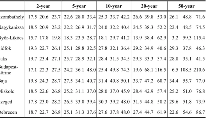
Having the parameters of the GEV distribution, the return values and related 95% confidence intervals were computed. The 2-year, 5-year, 10-year, 20-year, and 50-year return levels together with the lower bound and upper bound of the interval where the return level lies in with p=0.95 probability can be found in Table 2. As the time interval is increasing, the range of the confidence are widening. For the 5-year return period (which is the usual time interval for designing the sewerage system in urban environment) the estimated return values are between 23.5 mm and 36.1 mm, but the lowest upper bound of the 95%
confidence intervals is 28.7 mm (Table 2). In the case of the 50-year return period, the largest return values turned out to be at Győr-Likócs and Budapest- Lőrinc stations, where the ξ is a large positive value (see Table 1.). The confidence interval is extremely expanded in the case of the 50-year return level at Budapest-Lőrinc, whicht is a rural station in the capital. The return levels for very long return periods tends to enlarge the error due to inaccurate estimates of the shape parameters which describe the tails of a distribution. Generally, the confidence of the return levels decreases rapidly, when the return period is about two times longer than the length of the data series (Klein Tank et al., 2009).
Table 2. The return values of the 60-minute rainfall with the lower bound and the upper bound of the 95% confidence interval (mm)
2-year 5-year 10-year 20-year 50-year
Szombathely 17.5 20.6 23.7 22.6 28.0 33.4 25.3 33.7 42.2 26.6 39.8 53.0 26.1 48.8 71.6 Nagykanizsa 18.5 20.9 23.2 22.2 26.9 31.7 24.0 32.2 40.4 24.5 38.3 52.2 22.4 48.5 74.5 Győr-Likócs 15.7 17.8 19.8 18.3 23.5 28.7 18.1 29.7 41.2 13.9 38.4 62.9 3.2 59.3 115.4 Siófok 19.3 22.7 26.1 25.1 28.8 32.5 27.8 32.1 36.4 29.2 34.9 40.6 29.3 37.8 46.3 Paks 19.7 23.4 27.1 25.7 28.9 32.1 28.4 31.5 34.5 29.3 33.3 37.4 28.8 35.1 41.5 Budapest-
Lőrinc 17.1 22.3 27.5 24.2 36.1 48.0 25.4 49.8 74.3 19.6 68.1 116.5 6.5 108.5 210.6 Baja 19.8 24.3 28.7 27.5 34.1 40.7 31.4 40.8 50.1 33.7 47.2 60.7 34.4 55.7 77.0 Miskolc 18.5 22.6 26.8 25.2 31.1 37.0 28.0 37.0 45.9 28.4 42.9 57.4 25.2 51.0 76.8 Szeged 17.8 23.0 28.2 26.5 33.0 39.4 30.3 39.2 48.0 31.5 44.8 58.2 29.6 51.8 73.9 Debrecen 18.7 22.7 26.8 25.1 31.3 37.6 27.6 37.8 48.0 27.4 44.7 61.9 22.6 54.6 86.7
The return levels, or design values are often expressed in terms of rainfall intensity (mm/h) rather than rainfall depth (mm) over a certain duration in construction engineering. The latter has been chosen here, because this is what is actually measured at the meteorological stations.
5. Conclusion
This study focused on the short-term precipitation that is essential for hydrological planning. Hourly, namely 60-minute maximum precipitation series were analyzed from 96 stations operated by the Hungarian Metrological Service.
The return values are widely used parameters in planning, for example in construction of drainage systems. The return value can be determined as a value that is expected to occur on average once during the return period. To give an estimation for return values, the general extreme value distribution fitting is an adequate procedure. The 60-minute yearly maxima follow the GEV distribution and also the Gumbel fit suits to the sample series from all 96 stations. The spatial patterns of the return values for 2, 4, 5, 10, 20, 50 years coming from the GEV fit are similar. The influence of the orographic effect turns up in the Transdanubia region and in the territory of the North Hungarian Range, although greater values appear also in the plain regions in the southeastern part of Hungary. The 95% confidence intervals were computed to illustrate the uncertainty of the rainfall estimates to various return periods. Naturally, as the return period is increasing the range of the confidence are widening.
The methodology introduced here can be applied in the future for the renewing of the existing design criteria for infrastructure. The uncertainty can be decreased with using longer data series for estimation of the parameters of the GEV distribution. The series of automatic measurements can be lengthened for about a dozen of stations by the measurements rescued from the ombrograph registering papers after eliminating the inhomogeneity caused by the different sampling. Estimation of areal precipitation return levels by applying regional GEV distribution (Stedinger et al., 1993) is one of the possible directions of the continuation of our examinations. The methodology for estimating extreme areal precipitation by shifting the station-based precipitation to areal precipitation from the grid-based (Dyrrdal et al., 2016) also an option to consider.
References
Alexander, L., Zhang, X., Peterson, T., Caesar, J., Gleason, B., Klein Tank, A., Haylock, M., Collins, D., Trewin, B., Rahimzadeh, F., Tagipour, A., Ambenje, P., Rupa Kumar, K., Revadekar, J., and Griffiths, G., 2006: Global observed changes in daily climate extremes of temperature and precipitation. J. Geophys. Res. 111: D05,109. https://doi.org/10.1029/2005JD006290
Allen, M. and Ingram, W., 2002: Constraints on future changes in climate and the hydrologic cycle.
Nature 419, 224–232. https://doi.org/10.1038/nature01092
Anderson, T.W. and Darling, D.A., 1954: A test of goodness of fit. J. Amer. Statistic. Assoc. 49, 765–769.
https://doi.org/10.1080/01621459.1954.10501232
Besselaar, E.J.M. van den, Klein Tank, A.M.G., and Buishand, T.A., 2013: Trends in European precipitation extremes over 1951-2010. Int. J. Climatol. 33, 2682–2689.
Coles, S., 2001: An introduction to statistical modeling of extreme values. Springer Series in Statistics.
London: Springer-Verlag, 45–57. https://doi.org/10.1007/978-1-4471-3675-0_3
Coles, S. and Pericchi, L., 2003: Anticipating catastrophes through extreme value modelling. Appl.
Statistics 52, 405–416. https://doi.org/10.1111/1467-9876.00413
Coles, S., Pericchi, L.R., and Sisson, S., 2003: A fully probabilistic approach to extreme rainfall modeling. J. Hydrol. 273, 35–50. https://doi.org/10.1016/S0022-1694(02)00353-0
Chow, V.T., Maidment, D.R., and Mays, L.W., 1988: Applied Hydrology. McGraw-Hill. New York.
Chen, G. and Balakrishnan, N., 1995: A General Purpose Approximate Goodness-of-Fit Test. Journal of Quality Technology 27, 154–161. https://doi.org/10.1080/00224065.1995.11979578
Cunnane, C., 1989: Statistical Distributions for Flood Frequency Analysis, WMO-report no. 781 (Operational Hydrology Report no. 33), 73 pp. + 42 pp. appendix
Dyrrdal., A.V., Skaugen, T., Stordal, F. and Førland, E.J., 2016: Estimating extreme areal precipitation in Norway from a gridded dataset. Hydrol. Sci. J. 61, 483–494
https://doi.org/10.1080/02626667.2014.947289
Faragó, T., 1989: Extreme value analysis and some problems of applications in meteorology.
Meteorological Studies 64, Hungarian Meteorological Service. Budapest.
Faragó, T., Dobi, I., Katz, R. W. and Matyasovszky I., 1989: Meteorological application of extreme value theory: Problems of finite, dependent and non-homogeneous samples. Időjárás 93, 261–274.
Faragó, T. and Katz, R.W., 1990: Extremes and design values in climatology. WMO, TD-No. 386, Geneva.
Fowler, H. and Kilsby, C., 2003: A regional frequency analysis of United Kingdom extreme rainfall from 1961 to 2000. Int. J. Climatology 23, 1313–1334. https://doi.org/10.1002/joc.943
Gayer, J. and Ligetvári, F., 2006: Települési vízgazdálkodás csapadékvíz elhelyezés, VITUKI, Budapest, 76–90. (in Hungarian)
Groisman, P., Knight, R., Easterling, D., Karl, T., Hegerl, G., and Razuvaev, V., 2005: Trends in intense precipitation in the climate record. J. Climate 18, 1326–1350.
https://doi.org/10.1175/JCLI3339.1
Gumbel, E.J., 1958: Statistics of Extremes, Columbia University Press.
https://doi.org/10.1175/JCLI3339.1
Hailegeorgis, T.T., Thorolfsson, S.T., and Alfredsen, K., 2013: Regional frequency analysis of extreme precipitation with consideration of uncertainties to update IDF curves for the city of Trondheim.
J. Hydrol. 498, 305–318. https://doi.org/10.1175/JCLI3339.1
Jenkinson, A.F., 1955: The frequency distribution of the annual maximum (or minimum) values of meteorological events. Quart. J. Roy. Meteorol. Soc. 81, 158–172.
https://doi.org/10.1002/qj.49708134804
Katz, R.W., Parlange, M.B., and Naveau, P., 2002: Statistics of extremes in hydrology. Adv.Water Res.
25, 1287–1304. https://doi.org/10.1016/S0309-1708(02)00056-8
Kysely, J., 2009: Trends in heavy precipitation in the Czech Republic over 1961–2005. Int. J.
Climatol. 29, 1745–1758. https://doi.org/10.1002/joc.1784
Klein Tank, A.M.G., Zwiers, F.W. and Zhang, X., 2009: Guidelines on Analysis of extremes in a changing climate in support of informed decisions for adaptation. Climate Data and Monitoring WCDMP-No. 72, WMO-TD No. 1500, 56pp.
Klein Tank, A.M.G. and Konnen, G., 2003: Trends in indices of daily temperature and precipitation extremes in Europe, 1946–99. J. Climate 16, 3665–3680
https://doi.org/10.1175/1520-0442(2003)016<3665:TIIODT>2.0.CO;2
Klein Tank, A.M.G., Wijngaard, J., Konnen, G., Bohm, R., Demarree, G., Gocheva, A., Mileta, M., Pashiardis, S., Hejkrlik, L., Kern-Hansen, C., Heino, R., Bessemoulin, P., Muller-Westermeier, G., Tzanakou, M., Szalai, S., Palsdottir, T., Fitzgerald, D., Rubin, S., Capaldo, M., Maugeri, M., Leitass, A., Bukantis, A., Aberfeld, R., van Engelen, A., Forland, E., Mietus, M., Coelho, F., Mares, C., Razuvaev, V., Nieplova, E., Cegnar, T., Antonio Lopez. J., Dahlstrom. B., Moberg, A., Kirchhofer, W., Ceylan, A., Pachaliuk, O., Alexander, L., and Petrovic, P., 2002: Daily
dataset of 20th-century surface air temperature and precipitation series for the European Climate Assessment. Int. J. Climatology 22, 1441–1453. https://doi.org/10.1002/joc.773
Klok, E. and Klein Tank, A.M.G., 2008: Updated and extended European dataset of daily climate observations. Int. J. Climatology 29, 1182–1191. https://doi.org/10.1002/joc.1779
Koutsoyiannis, D. and Baloutsos, G., 2000: Analysis of a long record of annual maximum rainfall in Athens, Greece, and design rainfall inferences. Nat. Hazards 22, 29–48.
https://doi.org/10.1023/A:1008001312219
Koutsoyiannis, D., 2004: Statistics of extremes and estimation of extreme rainfall: I. Theoretical investigation. Hydrol. Sci. J. 49, 575–590. https://doi.org/10.1623/hysj.49.4.575.54430
Lakatos, M. and Matyasovszky, I., 2004: Analysis of the extremity of precipitation intensity using the POT method. Időjárás108, 163–171.
Lakatos, M. és Hoffmann, L., 2019: Növekvő csapadékintenzitás, magasabb mértékadó csapadékok a változó klímában. In (ed. Bíró, T.) Országos Települési Csapadékvíz-gazdálkodási Konferencia tanulmányai. 8-16. ISBN 978-615-5845-22-2 (in Hungarian)
https://vtk.uni-nke.hu/document/vtk-uni-nke-hu/K%C3%A9zik%C3%B6nyv_csapad%C3%A9k.pdf Łupikasza, E., Hansel, S., and Matschullat, J., 2010: Regional and seasonal variability of extreme
precipitation trends in southern Poland and central-eastern Germany 1951–2006. Int. J.
Climatol. 31. 2249–2271. https://doi.org/10.1002/joc.2229
Madsen, H., Pearson, C.P. and Rosbjerg, D., 1997: Comparison of annual maximum series and partial duration series methods for modeling extreme hydrologic events 2. Regional modeling. Water Resour. Res. 33, 759769. https://doi.org/10.1029/96WR03849
Marsaglia, G., 2004: Evaluating the Anderson-Darling Distribution. J. Statistic. Software 9, 730–737.
https://doi.org/10.18637/jss.v009.i02
Matyasovszky I., 2002: Statisztikus klimatológia. ELTE Eötvös Kiadó, Budapest. (In Hungarian) Moberg, A., Jones, P., Lister, D., Walther, A., Brunet, M., Jacobeit, J., Alexander, L., Della-Marta, P.,
Luterbacher, J., Yiou, P., Chen, D., Klein Tank, A., Saladie, O., Sigro, J., Aguilar, E., Alexandersson, H., Almarza, C., Auer, I., Barriendos, M., Begert, M., Bergstrom, H., Bohm, R., Butler, C.J., Caesar, J., Drebs, A., Founda, D., Gerstengarbe, F., Micela, G., Maugeri, M., Osterle, H., Pandzic, K., Petrakis, M., Srnec, L., Tolasz, R., Tuomenvirta, H., Werner, P., Linderholm, H., Philipp, A., Wanner, H. and Xoplaki, E., 2006: Indices for daily temperature and precipitation extremes in Europe analyzed for the period 1901–2000. J. Geophys. Res. 111, https://doi.org/10.1029/2006JD007103
Prescott, P. and Walden, A.T., 1980: Maximum likelihood estimation of the parameters of the generalized extreme value distribution. Biometrika 67, 723–724.
https://doi.org/10.1093/biomet/67.3.723
Pujol, N., Neppel, L., and Sabatier, R., 2007: Regional tests for trend detection in maximum precipitation series in the French Mediterranean region. Hydrol. Sci. J. 52, 956–973.
https://doi.org/10.1623/hysj.52.5.956
R Core Team, 2012: R: A language and environment for statistical computing. R Foundation for Statistical Computing, Vienna, Austria. ISBN 3-900051-07-0, URL http://www.R-project.org/
Stedinger, J. R., Vogel, R. M., and Foufoula-Georgiu, E., 1993: Frequency analysis of extreme events, In: D. R. Maidment (ed.), Handbook of Hydrology, McGraw-Hill, New York, 18.1–18.66.
Stephens, M.A., 1986: Tests Based on EDF Statistics. In (eds. D'Agostino, R.B.; Stephens, M.A.) Goodness-of-Fit Techniques. New York: Marcel Dekker. ISBN 0-8247-7487-6.
Stephens, M.A., 1970: Use of the Kolmogorov-Smirnov, Cramer-von Mises and related statistics without extensive tables. J. Roy. Statistic. Soc., Series B, 32, 115-122.
https://doi.org/10.1111/j.2517-6161.1970.tb00821.x
Szentimrey, T., 1999: Multiple Analysis of Series for Homogenization (MASH). Proceedings of the Second Seminar for Homogenization of Surface Climatological Data, Budapest, Hungary;
WMO, WCDMP-No. 41, 27–46.
Varga, L., Buzás, K. és Honti, M., 2016: Új csapadékmaximum-függvények. Hidrológiai Közlöny 96, 64–69. (in Hungarian)
Váradi, F. and Nemes, Cs., 1992: Rövid időtartamú csapadékmaximumok gyakorisága Magyarországon. Légkör XXXVII. 3, 8–13. (In Hungarian)
Venema, V., Mestre, O., Aguilar, E., Auer, I., Guijarro, J.A., Domonkos, P., Vertacnik, G., Szentimrey, T., Štěpánek, P., Zahradnicek, P., Viarre, J., Müller-Westermeier, G., Lakatos, M., Williams, C.N., Menne, M., Lindau, R., Rasol, D., Rustemeier, E., Kolokythas, K., Marinova, T., Andresen, L., Acquaotta, F., Fratianni, S., Cheval, S., Klancar, M., Brunetti, M., Gruber, C., Duran, M.P., Likso, T., Esteban, P. and Brandsma,T., 2012: Benchmarking monthly homogenization algorithms. Climate Past 8, 89–115. https://doi.org/10.5194/cp-8-89-2012
Wilks, D.S., 1993: Comparison of three-parameter probability distributions for representing annual extreme and partial duration precipitation series. Water Resour. Res. 29, 3543–3549.
https://doi.org/10.1029/93WR01710
Willett, K., Jones, P., Gillett, N., and Thorne, P., 2008: Recent changes in surface humidity:
development of the HadCRUH dataset. J. Climate 21, 5364–5383.
https://doi.org/10.1175/2008JCLI2274.1
Zolina, O., Simmer, C., Belyaev, K., Kapala, A., and Gulev, S., 2009: Improving estimates of heavy and extreme precipitation using daily records from European rain gauges. J. Hydrometeorol. 10, 701–716. https://doi.org/10.1175/2008JHM1055.1