DOI:10.28974/idojaras.2018.3.7
IDŐJÁRÁS
Quarterly Journal of the Hungarian Meteorological Service Vol. 122, No. 3, July – September, 2018, pp. 345–360
A dynamic data-driven forecast prediction methodology for photovoltaic power systems
Zoltán Kapros
Szent István University, Faculty of Mechanical Engineering,
Institute of Environmental Systems, Department of Physics and Process Control, Páter Károly u. 1., Gödöllő, H-2103, Hungary,
E-mail: zkapros@t-online.hu
(Manuscript received in final form July 31, 2017)
Abstract⎯At present, the capacity of the new photovoltaic (PV) systems are growing rapidly in Hungary. The limit to growth can be estimated, but it is influenced by several things. Even a realistic goal for the next 20–30 years can be to reach the 20–25% variable renewable energy ratio in the electricity consumption. The main barrier is the variability of these systems, thus the grid integration is a huge challenge in the near future. A new dynamic data-driven forecasting methodology is worked out and tested by examining the Budapest District Heating Co. Ltd. top installed solar systems. The tested prediction method was only for 5 minutes ahead in the expected average performance in a 15-minute period. The main elements of the tested methodology and some main results will be presented in this article.
Key-words: small scale photovoltaic systems, genetic algorithm, dynamic data driven forecast, equivalent peak load hour, power prediction
1. Introduction
The aim of the Hungarian National Energy Strategy is that the annual final energy consumption school dot exceed 692 PJ by 2030 compared to the 677 PJ/year in 2012 (Parliamentary Decision 77/2011). According to the National Environmental Programme, in the field of renewable energy sources in Hungary, it is desirable to put greater emphasis on decentralized, local
applications, in particular in relation to solar energy (Parliamentary Decision 27/2015). In addition, the main national energy target is also fixed in this Decision by 2020. Therefore, the targeted share of renewable energy sources is 14.65%, and the total reached energy savings could be 10% with environmental considerations. However, our national commitment towards the European Union is ‘only’ 13% share (Directive 2009/28/EC). In Hungary, the share of renewable energy has already reached 9.51% in 2014 (Szabó, 2016). For the 13% share in the period in 2015–2020 we have already reached 37% increase from the 2014 level, but for the national target are still need 49% growing, if the country's gross energy consumption will not increase until 2020.
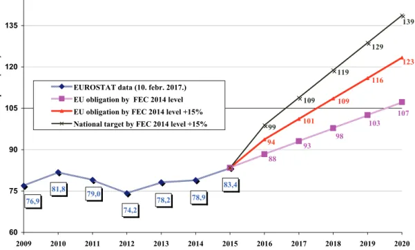
The individual Member States data of the renewable energy utilization can be traced from the Eurostat public databases (Eurostat Database, 2017). At the end of 2014, the renewable energy ratio was found to be 9.5% of the total energy consumption. Fig. 1 shows the changes in the renewable energy consumption achieved in Hungary compared to the 2009 data. Overall, we can see that near 10% gross inland renewable energy consumption growth is achieved in the previous six years. Now it seems, that at least nearly 30%
surplus could be needed over the next five years. The obligated amount depends on the final energy consumption (FEC) in 2020. If it would be only 15% higher than it was in 2014, we would need near 40% growing until 2020. Moreover, the national target is higher than the EU obligation. All in all, this seems a serious challenge.
Fig. 1. Changes in renewable energy consumption in Hungary.
81,8
76,9 79,0
74,2
78,2 78,9
83,4
88 93
98
103 107
94
101 109
116 123 139 129 119
109 99
60 75 90 105 120 135
2009 2010 2011 2012 2013 2014 2015 2016 2017 2018 2019 2020
Gross inland RES consumption [PJ/a]
EUROSTAT data (10. febr. 2017.) EU obligation by FEC 2014 level EU obligation by FEC 2014 level +15%
National target by FEC 2014 level +15%
However, it is important to point out that the share of the renewable energy in Hungary has been significantly modified from March 14, 2017, after the domestic energy methodologies update (Eurostat Database, 2017). Thus, the official share of renewable energies has increased to 14.6% in 2014 from the earlier presented 9.51%. Therefore, it seems presently, that Hungary was able to reach the renewable target without serious progress or greater emphasis on decentralized, local applications.
Although, in 2015, the volume of electricity in the Hungarian feeding tariff system increased only by 1.1% (reaching the 25 MW PV capacity), due to the support system restructuring, significant growth is expected in 2016–2017 by the PV systems. Thus, more than 1.5 GW PV capacity is possible until 2018 due to new local applications. More weather-dependent power plants (variable energy resources) and complex development are needed. By the mitigation of the growing development and operational costs because of the larger variable energy production, one of the key elements is the predictability.
It is important to see that there are huge differences between the different types of variable energy resources. Solar energy utilization is fundamentally governed by planetary conditions. Thus, a theoretically expected solar power curve as a guideline can be specified. However, the actual differences in meteorological conditions can cause significant differences in the power outputs from the PV systems. Besides the intensity of the light, the actual spectral composition of the sunshine also determines the actual power generation capacity of the solar cells. In case of small rooftop systems these effects are not measurable cost-effectively because of the relative very small produced energy amounts, and the real time data management also would be relatively expensive by one or more small PV systems. At the same time, unexpectable changes in the spectral composition and other important effects (e.g., air temperature) give information, if we have a god theoretical reference curve. So the light also could be an information carrier.
In clear weather, with the greatest direct radiation ratio, the largest part of the intensity of the global radiation could produce electricity with photovoltaic effect, so this situation is more or less predictable. In cloudy weather, the indirect (diffuse) radiation component increases the spectral characteristics of the radiation changes, and the predictability declines. The differences in meteorological effects (the ratio between the direct and indirect components and spectral characteristics in the solar radiation or temperature conditions) from the expected values in the near past could give information for the near future. In this case, the main task of meteorological measurements can be to sign the huge changes in circumstances. Therefore, this could indicate if the information in the light from the near past is not or only partly applicable to predict the near future.
2. Assessment
The latest generation of prediction methods works with a number of meteorological, temporal, and geographic parameters, such as temperature, relative humidity, wind speed, sunshine duration (SSD), day of the year, and location (latitude, longitude, and altitude) that affect the global radiation modeling values. A recent prediction method is generally based on artificial neural networks, where the expected net global radiation could be predicted by the values of these parameters (Hussain and Al-Alili, 2015). So the predictions are generally based on the experienced data and local knowledge. The so-called typical meteorological year is built of many time series parameters. The resulting values give a good approach in terms of long-term durability, but in terms of a given year, there may be significant inaccuracies. A further disadvantage is that the global and local environmental changes are not built into the calculations. Thus, analysis of trends and outline additional parameters are also required. These are very expensive methods.
As a new direction, the typical meteorological year is determined only from easily and cheaply available data, but this simplified data set can only be treated as a first approximation, and the forecast can be based on the variation of this data set and some dynamically measured parameters (actual whether parameters). In the University of Leeds, the global radiation quantity with one minute dividing was predicted in this way (Bright at al, 2015). Developing the conditions for determining the accurate prediction of solar power systems considered to be a key factor contributing to the integration to the electricity network (Lorenz and Heinemann, 2012). By the optimal grid control and balancing activities, the relative error of short-term forecasting of energy production should be below 10% (Wu and Xia, 2015). A reliable network operation requires different forecast horizons (Kostylev and Pavloski, 2011).
These aims can be categorized as follows:
1. planning, optimization, network assessment, cost-benefit analysis, evaluation of alternatives, verification by supports;
2. 15 minutes schedule giving an electricity trader;
3. clarification of the planned schedule before the beginning of the relevant period;
4. clarification of the planned schedule within the relevant 15-minute-long period;
5. prediction for a very short (balancing) forecast, for example only 1 minute ahead.
The demand for forecasts for shorter periods first appeared by the larger photovoltaic power generation systems. For larger PV plants, the cloud migration and its impact on the intensity changes can be followed. The average
intensity in an area can be estimated with moving averages of the radiation profiles (spatial smoothing effect) (Longhetto et al., 1989). The solar energy prediction by the high PV power plants can be managed by a wavelet variability model which uses 25 radiometer sensors around the plant (Dyreson at al., 2014).
Solutions like the wavelet variability model, which are acceptable for multi- megawatt power plants (Lave et al., 2013) even often do not provide cost effective solution for small scale sizes. This paper examines the possibilities suggested by the last two points and illustrates some of the results (Kapros, 2017).
3. Methods 3.1. Individual prediction of PV systems
Modeling the PV predictions could be based on stochastic assessments.
However, the variability of PV generation does not follow any well described distribution. The stochastic models, which use standard or other type distributions, can be used for several hours, several days, or even longer period.
Furthermore, it is not enough to know of the average external temperature conditions, because the PV system efficiency is determined also by other external parameters (e.g., spectral light irradiation, temporary cloud effects, etc.), and by the individual characteristics of the PV systems. For these reasons, the genetic algorithm method was applied in this study.
A genetic algorithm approach is based on the observed mathematical regularities of genetic populations. Accordingly, the knowledge on the observed capabilities (as genetically determined values) in the starting position can determine the possibilities of the future capabilities in the probability space.
Therefore, performance, which has the highest probability within a given set of possibilities, can be precisely defined.
The genetic method was performed with an encoding process in the sampling period and a decoding process in the predicted period based on deviations between the typically expected and the measured real performance values. Thus, the fundamental part of this methodology was the developing of the expected typical performances for every minute in the examined period with physically based forecasts achievable free of charge. For getting the expected typical data some well-known equations for calculating the amount o electricity with relatively few required information and some free public databases were used. Therefore, for every minute of a year, the expected performance values were determined in a reproducible manner. The amount of electricity, generated by a photovoltaic system, is expressed by the following equation based on the effective global radiation (Earthscan, 2008):
, M PV
el H A
q = αβ ×η × , (1)
where qel is the photovoltaic power generation capacity [W], Hα,β is the effective radiation with α tilt angle and β orientation of the PV modules[W/m2], ηM is the PV module efficiency [%], and Apv is the useful photovoltaic solar surface [m2].
The aim of this study was to find results which are independent from the PV generators. For this reason, the equivalent peak load hours were calculated.
Therefore, the codes which are used in the genetic algorithms were developed from the expected equivalent peak load hours based on physical modeling by typical conditions. The equivalent peak load hours (Sharma and Tiwari, 2012) are characterized by the energy-generating capacity in a given moment. It means that, if the same amount of power will produce in one year, the equivalent peak load hours are equal to the traditional peak load hours:
.
P real
ekv P
h =ζ
(2) The dimension of the equivalent peak load hour (hekv) could be kWh/kW or hour. This is the ratio of a typical solar electricity generating capacity of a given t period (ξreal [kWh]) and the nominal capacity of the PV system (Pp [kWp]. If the performance is expressed as an equivalent peak load hour, the expected value can be written as follows:
), )
( ) ( ) (
, (
P
PV t PV
ekv P
A t t t G
h = ×η × (3)
where Gpv [W/m2] is the sum of the effective global radiation (effective direct normal to the plain) and diffuse solar radiation by south orientation. The equivalent peak load hours show a reachable capacity at a given moment. If the system is functioning at a given time at specific equivalent peak load hours, then in an imagined year with equal continuous output power, the same value would result for the peak load hours for that year. This value represents an actual capacity of the PV power plant, which is clear, meaningful, and comparable.
Therefore, in every minute, we can get the expected equivalent peak load hours according to the following equation:
. ) 8760 1000 (
) ) (
, ( ×
= ×
p AC AC
ekv P
t t P
h (4)
Therefore, it is enough to make a physically based model for the PV generator’ expected alternating current performance at a given time (PAC [W]), and this is easy to express this value in equivalent peak load hours. The invented
new method is a data-driven determination system, where expected values are physically modeled as in the forecasted time (t0), ehen they are dynamically and continuously changing depending on the sets of measured data in the monitoring period before t0 with Δt1, Δt2, ..., Δtn durations. This continuous changing is guided by the encoded metered data contents of the sampling period, which express also the currently unique and determinative effects for the electricity production. Therefore, the coding system is capable to capture the slightly or seriously unexpected behavior (the differences) in the sampling period as genetically deterministic properties. In this coding system, there are stock defined unique properties, and this gives the approximately parental genetic material. Thus, the code most likely and valid in the following short time can be determined.
All in all, the probability of any next value can be calculated within the range which is designated by the recorded code set in the sampling period. This makes it possible to join different probabilities for different amounts of the future performances. However, the chances still remain for the decisive changes in extreme weather conditions. These effects are considered as genetic mutation effects. The mutation gives a performance, which has zero probability based on the genetic material of the sampling period. The above is determined by the differences between the observed (measured) and expected equivalent peak load hours according to the next equation:
) , (
)) ( ) ( ) (
( *
*
t h
t h t t h
H
i i
i = i − (5)
where the expected equivalent peak load hours (h*i) are determined by the physical-based modeling and analysis. The real equivalent peak load hours (hi) can be calculated from the measured performance values. The difference between these two values is the physically based prediction error, from which the specific error (Hi) was expressed. The past series of this specific error may also be defined in accordance with the Eq. (6) in the sampling period (before t time moment, between n and m time moments). From these, the average dH/dt change can be determined. In the following equation, the time is in seconds units according to the SI system:
). (
...
) (
)
60( 1 1 2 1
m n
m m
i i
i i i
i
t
H H
H H
H H t
H dt
dH
−
+
−
−
−
Δ
+ +
+
− +
= − Δ
≈ Δ (6)
In Eq. (6), the length of the periods between Hi and Hm are the same according to the following equation:
.
... 1
2 1
1 i i m m
i
i t t t t t
t − − = − − − = = + − (7)
Thus, the error factor prediction is described as follows:
. ) 1
( )
1 ( ) 1
( 60 0,4 60
1
n t n
t t
i i
t i i
t
t t
H H dt
H dH dt
H dH
H − −
Δ Δ
− Δ
+Δ
≈ +
≈ +
= (8)
The 0.4 multiplier exponent was the most favorable during the test of Eq. (8). The reason is that the H specific errors during the sampling period are not fully independent from each other. Behind the variations of these specific error values, more stochastic processes can be assumed in the sampling period.
Changing of the specific errors between the predicted and measured values in the period between m and n is made only partly by those natural effects, which occurs similarly after the t-n period in t time. Thus, the predicted equivalent peak load hours (κt) for t time at n time can be calculated by the following equation:
) 1
* (
*
*
t t
t t t
t =h +H ×h =h × +H
κ . (9)
In the research, the duration of the predicted period was 1 minute, the n exponent was 5 minutes, and the m exponent was 15 minutes. Therefore, during the measurement and analysis, the series of κt was available 5 minutes before time t. This gave the opportunity to give a different forecast for the average performance in every 15 minutes with 5 minutes before the end of the period.
During the test, the prediction for average performance (equivalent peak load hours) in 15-minute periods based on 5 minutes measured data and 10 minutes predicted data from this presented method. Thus, the predicted 15-minute average data of the average equivalent peak load hours in the given Δt period (κq [h]) is illustrated with the following equations:
).
10 ( ) 11 ( ) 12 ( ) 13 ( ) 14 (
1= t− + t− + t− + t− + t−
q h h h h h
h (10)
) .
1 ( ) 2 ( ) 3 ( ) 4 ( ) 5 ( ) 6 ( ) 7 ( ) 8 ( ) 9 (
2 t t t t t t t t t t
hq =κ − +κ − +κ − +κ − +κ − +κ − +κ − +κ − +κ − +κ (11) 15 .
) ( ) ) (
( h1 t h 2 t
t q q
q
= +
κ (12)
The significance of the error factor is stronger in these times when the radiation is more intensive, so the period between 10:00 and 16:00 in local time were also separately analyzed.
3.2. Virtual PV systems group prediction
The second part of this research examined the prediction possibilities for the virtual groups based on the former methodology. The prediction is based on
only one real-time monitored photovoltaic (VP) power plant, but the predicted performances were made related to the whole virtual PV power system. This methodology could be useful for some very small (micro) domestic PV systems which are built in a small region. In view of the methodology, the forecasting error between the analytical prediction and the real energy production in a 15 minutes period by a monitored plan could correlate to this error by the other power plant. This correlation is determined by the following equation:
) (
) ( ) 1 (
) ) (
( *
* 1 1
t t h t
t t h
qt qt qt
q q
κ κ κ
− −
≈ . (13)
In the case of virtual a generator built by w+1 number of PV systems, the forecasts can be calculated with the weighted (as rated power) predictions by systems. So the virtual-group level forecast could be given by the following equation:
Pw P
P P
qw Pw q
P q
P qt
P
qt I I I I
t I
t I
t I t t I
+ + + +
+ + +
= +
Κ ...
) ( ...
) ( )
( )
) ( (
2 1 0
2 2 1
1
0κ κ κ κ
, (14)
where the IP0 is the rated power of that reference PV power system, which is alone monitored directly and in real time by the whole virtual group.
3.3. Measurement
The test system was the solar power system of the FŐTÁV Ltd., which is built on the top of its central office building by 150 pieces of PV panels with 250 WP
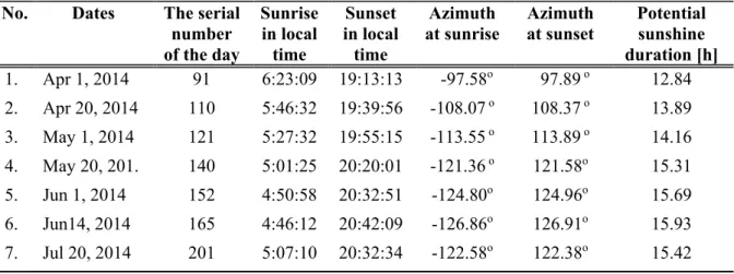
nominal rated capacities per units and eight inverters, which connect it to the public grid. The maximum output capacity of one inverter is 5 kW, and in six cases there are a ten solar panels formed string and a nine solar panels formed string parallel connected, and in two cases there are two parallel connected nine panel formed sting behind an inverter. Based on the measurement data of these eight inverters we could evaluate eight independent systems. The types of PV modules are AS-250 W 60P ECO polycrystalline silicon solar cells. The orientations of PV modules are +10.7 degrees (SSW), and their tilt angles are 20 degrees. The nominal connection capacity of the whole PV plants to the grid is 40 kW. The research examined a reference power plant owned by the Budapest District Heating Co. Ltd. The PV plant is located in the company’s headquarter in Budapest on the top of the ‘D’ building. The research analyzed data from seven different days which was randomly selected (Table 1).
Table 1. The test days and characteristics No. Dates The serial
number of the day
Sunrise in local time
Sunset in local time
Azimuth at sunrise
Azimuth at sunset
Potential sunshine duration [h]
1. Apr 1, 2014 91 6:23:09 19:13:13 -97.58o 97.89 o 12.84 2. Apr 20, 2014 110 5:46:32 19:39:56 -108.07 o 108.37 o 13.89 3. May 1, 2014 121 5:27:32 19:55:15 -113.55 o 113.89 o 14.16 4. May 20, 201. 140 5:01:25 20:20:01 -121.36 o 121.58o 15.31 5. Jun 1, 2014 152 4:50:58 20:32:51 -124.80o 124.96o 15.69 6. Jun14, 2014 165 4:46:12 20:42:09 -126.86o 126.91o 15.93 7. Jul 20, 2014 201 5:07:10 20:32:34 -122.58o 122.38o 15.42
The reference power plant was considered only one part of the whole system (one inverter part Eq. (8)). With the same orientation and the same angle, 19 panel units have a single inverter. The main data of the plant are:
- Latitude: 47.4584oN, Longitude: 19.045oE;
- PV module type: AS-60P 250 W ECO;
- Rated power of a panel: 250 Wp;
- The number of solar panels installed: 150;
- Position: +10.7 degrees (SSW) (determined by measuring from map);
- Angle of inclination: 20 degrees;
- The PV power plant nominal connection capacity: 40 kW.
The group forecast is based on the measurement and forecast data of a single system. Two PV generator groups with different characters were made virtually. The homogeneous group was the photovoltaic system of the FŐTÁV in the Kalotaszeg street as a whole (eight independent and measured inverter units). The heterogeneous group was built partly from the homogeneous virtual group. It contained the number 1, the number 3 (both 4750 WP), and the number 7 (4500 WP) inverters, but partly it was consisted of two other small scale PV systems with different locations and products (both 2160 WP). Table 2 shows the main data.
Table 2. The homogeneous and the heterogeneous groups Homo-
geneous group
Place Rated power Hetero- geneous
group
Place Rated power
Inv. 1. Kalotaszeg str. 4750 WP Inv. 1. Kalotaszeg str. 4750 WP
Inv. 2. Kalotaszeg str. 4750 WP Inv. 3. Kalotaszeg str. 4750 WP
Inv. 3. Kalotaszeg str. 4750 WP Inv. 7. Kalotaszeg str. 4500 WP
Inv. 4. Kalotaszeg str. 4750 WP HADR Hadriánusz str. 2160 WP
Inv. 5. Kalotaszeg str. 4750 WP LEIB Leibstück str. 2160 WP
Inv. 6. Kalotaszeg str. 4750 WP
Inv. 7. Kalotaszeg str. 4500 WP
Inv. 8 Kalotaszeg str. 4500 WP
Total rated power 37 500 WP Total rated power 18 320 WP
4. Measured data and statistical analysis
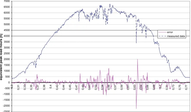
The results of the forecast by a clear sky are demonstrated in Fig. 2. The numerical error of the forecast is also important. The uncertainty effects are characterized, which are caused by the PV system in the network's stability (Fig.
2.). The dynamic forecast error in most cases is below 500 hours, and only one case was more than 2000 hours with a short oscillation. It seems that if the effect which caused the error and its length would be known, the forecast could be more accurate by attenuating the errors caused by oscillatio.
April 1, 2014 was the second least volatile day from the seven tested days, which was slightly cloudy, basically sunny, and there were stable light conditions. Predictability is difficult for these types of weather, because the bell curve is not clearly outlined, and significant differences may occur compared to the expected values. However, the changes in the lighting conditions are less dynamic, which is favorable in view of the developed genetic algorithm methodology. So the relative errors of the prediction between 10 and 16 hours were only typically below 5%. Furthermore, we noticed that some major faults, which caused by short-acting dynamic changes, can incorporate into the forecast. and later can cause an opposite distortion. In Fig. 2 the measured values and the experienced prediction errors of the equivalent peak load hours also are shown. The forecast distortion and oscillations are well-observed. For the oscillation damping. it may be sufficient to use some real-time measurement, of the typical conditions (light intensity, wind speed, spectral conditions), because the real-time tracking could be useful to filter the mutations effects out of their following there lifetime.
Fig. 2. AC error of the forecast, calculated by Eq. (9) on April 1, 2014.
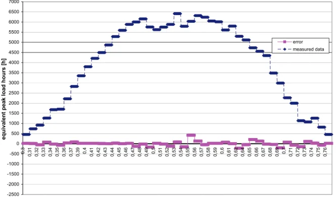
Figs. 3 and 4 show the relative error according to the prediction calculated by Eq. (12), where the forecast is for a 15 minutes average equivalent peak load hour and it was made also 5 minutes earlier, than the end of the period. In a highly volatile day, the method was also tested. Even in this case, the forecast accuracy was an average of around 9% (Fig. 5.)
Fig. 3. AC relative error of the forecast, calculated by Eq. (12) on April 1, 2014.
-2500 -2000 -1500 -1000 -500 0 500 1000 1500 2000 2500 3000 3500 4000 4500 5000 5500 6000 6500 7000
0,3 0,31 0,33 0,35 0,37 0,38 0,4 0,42 0,44 0,45 0,47 0,49 0,51 0,52 0,54 0,56 0,57 0,59 0,61 0,63 0,64 0,66 0,68 0,7 0,71 0,73 0,75 0,77
equivalent peak load hours [h] error
measured data
-30%
-20%
-10%
0%
10%
20%
30%
0,3 0,32 0,33 0,35 0,37 0,38 0,4 0,41 0,43 0,45 0,46 0,48 0,49 0,51 0,53 0,54 0,56 0,57 0,59 0,61 0,62 0,64 0,65 0,67 0,69 0,7 0,72 0,73 0,75 0,77
relatív error [%]
The average relative error between 10:00 – 16:00 was 1.55%.
Fig. 4. AC error of the forecast, calculated by Eq. (12) on April 1, 2014.
Fig. 5. AC error of the forecast,calculated by Eq. (12) on June 1, 2014.
Considering the researched seven days, the average relative error was below 6%. In three days of seven, all errors by each period between 10 and
-2500 -2000 -1500 -1000 -500 0 500 1000 1500 2000 2500 3000 3500 4000 4500 5000 5500 6000 6500 7000
0,3 0,31 0,32 0,33 0,34 0,35 0,36 0,37 0,39 0,4 0,41 0,42 0,43 0,44 0,45 0,46 0,47 0,48 0,49 0,5 0,51 0,52 0,53 0,54 0,55 0,56 0,57 0,58 0,59 0,6 0,61 0,62 0,64 0,65 0,66 0,67 0,68 0,69 0,7 0,71 0,72 0,73 0,74 0,75 0,76
equivalent peak load hours [h]
error measured data
-2500 -2000 -1500 -1000 -500 0 500 1000 1500 2000 2500 3000 3500 4000 4500 5000 5500 6000 6500 7000 7500 8000
0,31 0,32 0,33 0,34 0,35 0,36 0,37 0,39 0,4 0,41 0,42 0,43 0,44 0,45 0,46 0,47 0,48 0,49 0,5 0,51 0,52 0,53 0,54 0,55 0,56 0,57 0,58 0,59 0,6 0,61 0,62 0,64 0,65 0,66 0,67 0,68 0,69 0,7 0,71 0,72 0,73 0,74 0,75 0,76 0,77 0,78 0,79 0,8
equivalent peak load hours [h] error
measured data
16 hours were below 10%. On average of these seven days, the prediction errors remain below 5% with 65% probability.
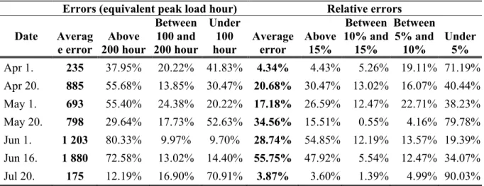
Based on the differences between the predicted values and the measurement data, the absolute and relative errors for each minutes were determined with the following equations. The results of the prediction are shown in Tables 3 and 4. The results of the forecast for virtual group in the tested day are shown in Table 5.
*.
* ,t t ekv
t h h
h = −
Δ (15)
. 100
,t ekv h t
h
h = × Δh (16)
Table 3. 1-minute forecast performance data between 10:00 and 16:00 hours Errors (equivalent peak load hour) Relative errors Date Averag
e error
Above 200 hour
Between 100 and 200 hour
Under 100 hour
Average error
Above 15%
Between 10% and 15%
Between 5% and 10%
Under 5%
Apr 1. 235 37.95% 20.22% 41.83% 4.34% 4.43% 5.26% 19.11% 71.19%
Apr 20. 885 55.68% 13.85% 30.47% 20.68% 30.47% 13.02% 16.07% 40.44%
May 1. 693 55.40% 24.38% 20.22% 17.18% 26.59% 12.47% 22.71% 38.23%
May 20. 798 29.64% 17.73% 52.63% 34.56% 15.51% 0.55% 4.16% 79.78%
Jun 1. 1 203 80.33% 9.97% 9.70% 28.74% 54.85% 12.19% 13.57% 19.39%
Jun 16. 1 880 72.58% 13.02% 14.40% 55.75% 47.92% 5.54% 12.47% 34.07%
Jul 20. 175 12.19% 16.90% 70.91% 3.87% 3.60% 1.39% 4.99% 90.03%
Table 4. 15-minute forecast performance data between 10:00 and 16:00 hours (5 minutes before the end of the period)
Absolute errors (equivalent peak load
hour) Relative errors
Date Average error
Above 200 hour
Between 100 and 200 hour
Under 100 hour
Average error
Above 15%
Between 10% and 15%
Between 5% and 10%
Under 5%
Apr 1 87 12.50% 25.00% 62.50% 1.55% 0.00% 0.00% 4.17% 95.83%
Apr 20 302 37.50% 16.67% 45.83% 6.63% 12.50% 0.00% 29.17% 58.33%
May 1 256 37.50% 29.17% 33.33% 5.92% 12.50% 8.33% 25.00% 54.17%
May 20 260 29.17% 8.33% 62.50% 4.36% 8.33% 8.33% 4.17% 79.17%
Jun 1 397 58.33% 20.83% 20.83% 9.29% 20.83% 12.50% 20.83% 45.83%
Jun 16 694 75.00% 8.33% 16.67% 13.09% 37.50% 12.50% 16.67% 33.33%
Jul 20 56 8.33% 4.17% 87.50% 0.93% 0.00% 0.00% 8.33% 91.67%
Table 5. 15-minute forecast performance data for a virtual power plan (5 minutes before the end of the period)
Date
Evaluated periods
Absolute errors
(equivalent peak load hour) Relative errors
2014 Homo-
geneous
Hetero- geneous
Homo- geneous
Hetero- geneous
Apr 1 7:08-18:36 79 89 3.01% 3.42%
10:00-16:00 90 102 1.60% 1.77%
May 20 6:25-19:09 473 331 9.78% 9.51%
10:00-16:00 665 466 9.65% 7.67%
Jun 1 7:34-19:14 273 429 11.28% 19.55%
10:00-16:00 402 567 8.94% 14.81%
Jul 20 6:32-19:14 61 161 1.86% 4.78%
10:00-16:00 80 214 1.31% 3.47%
Average whole daytime 222 253 6.48% 9.32%
10:00-16:00 309 337 5.38 6.93
5. Conclusions
The overall conclusion is that the developed dynamic prediction method appears to be an applicable method in case of the small-scale solar systems. It is verified that the prediction for each 15-minute period within five minutes before the end has a good accuracy even under strongly variable weather. Although the measurements were made by a relatively small system, the results get special actuality by the expected huge increases of the almost 500 kWP domestic photovoltaic systems. Thus, the applicability of this dynamic forecasting method for the individual larger system would be useful to test.
The presented group-level prediction method for the micro PV systems could be an essential tool for the so-called aggregator services, because they would be able to use this information with their demand side management activities for the timetable of the virtual smart grid.
The presented method is a good example for the less costly dynamic forecasting solution demonstrating, that the active measures with reasonable accuracy in most cases would be ensured.
References
Bright, J., Crook, R., and Taylor, P.G., 2015: Methodology to stochastically generate synthetic 1-minute irradiance time-series derived from mean hourly weather observational data. Proceedings of the ISES Solar World Congress 2015, Daegu, Korea, 08-12. November, 2015, 142–151.
Dyreson, A.R., Morgan, E.R., Monger, S.H., and Acker T.L., 2014: Modeling solar irradiance smoothing for large PV power plants using a 45-sensor network and Wavelet Variability Model.
Solar Energy 110, 482–495.
Directive 2009/28/EC of the European Parliament and of the Council of 23 April 2009 on the promotion of the use of energy from renewable sources and amending and subsequently. Annex I. National overall targets for the share of energy from renewable sources in gross final consumption of energy in 2020 repealing Directives 2001/77/EC and 2003/30/EC,
Earthscan, 2008: Planning and installing photovoltaic systems. A guide for installers, architects and engineers. Earthscan Publications Ltd.
Eurostat Database, Complete energy balances - annual data (nrg_110a). Downloading is on 10.
February 2017. http://appsso.eurostat.ec.europa.eu/nui/show.do?dataset=nrg_110a&lang=en Eurostat Database, Share of energy from renewable sources (nrg_ind_335a). Downloading is on 2.
May 2017. http://appsso.eurostat.ec.europa.eu/nui/show.do?dataset=nrg_ind_335a&lang=en Eurostat Database, Supply, transformation and consumption of renewable energies - annual data.
Downloading is on 10. February 2017.
http://appsso.eurostat.ec.europa.eu/nui/show.do?dataset=nrg_107a&lang=en
Hussain, S. and Al-Alili, A., 2015: Selection of relevant input parameters for solar radiation, ISES Solar World Congress, 8-12. November 2015, Daegu, Korea, 2 p. Downloading is on 10.
December 2015. http://swc2015.org/index.php?g_page=program&m_page=program11
Kapros, Z., 2017: Autonomous and grid collaborative photovoltaic system optimization. PhD thesis, Szent István University, Gödöllő.
Kostylev, V. and Pavlovski, A., 2011: Solar power forecasting performance towards industry standards.
Proceedings of the 1st International Workshop on the Integration of Solar Power into Power Systems, 24. October 2011, Aarhus, Denmark, 8 p. Downloading is on 28. December 2015.https://ams.confex.com/ams/92Annual/webprogram/Manuscript/Paper203131/AMS_VK_
%20AP_Paper%202011%20submitted.pdf
Lave, M., Kleissl, J. and Stein, J.S. 2013: A wavelet-based variability model (WVM) for solar PV power Plants, IEEE Trans. Sustain Energy 4, 501–509.
Longhetto, A., Elisei, G. and Giraud, C., 1989: Effect of correlations in time and spatial extent on performance of very large solar conversion systems, Solar Energy 43, 77–84.
Lorenz, E., and Heinemann, D., 2012: Prediction of solar irradiance and photovoltaic power. Compr.
Renew. Energy. 239–292.
Parliamentary Decision 77/2011 (X. 14.) about the implementation of the National Energy Strategy Parliamentary Decision 27/2015 (VI. 17.) about the National Environmental Programme for 2015-
2020
Sharma, R. and Tiwari, G.N., 2012: Technical performance evaluation of stand-alone photovoltaic array for outdoor field conditions of New Delhi. Applied Energy 92, 644–652.
Szabó, Zs., 2016: A megújuló energia termelés Magyarországon, A megújuló villamosenergia- támogatási rendszer (METÁR) jövőbeni keretei Magyarországon. REKK Energiapolitikai Fórum, 2016. június 9. Budapest. (In Hungarian). Downloading is on 15. December 2016.
http://rekk.hu/downloads/events/Sz.Zs._REKK_20160609_final.pdf
Wu, Z. and Xia, X., 2015: Optimal switching renewable energy system for demand side management.
Solar Energy 114, 278–288.