sciences
Article
A Fully Automatic Procedure for Brain Tumor Segmentation from Multi-Spectral MRI Records Using Ensemble Learning and Atlas-Based Data Enhancement
Ágnes Gy˝orfi1,2 , László Szilágyi1,2,3* and Levente Kovács1,3
Citation:Gy˝orfi, Á.; Szilágyi, L.;
Kovács, L. A Fully Automatic Procedure for Brain Tumor Segmentation from Multi-Spectral MRI Records Using Ensemble Learning and Atlas-Based Data Enhancement.Appl. Sci.2021,11, 564.
https://doi.org/10.3390/app11020 564
Received: 2 December 2020 Accepted: 1 January 2021 Published: 8 January 2021
Publisher’s Note: MDPI stays neu- tral with regard to jurisdictional clai- ms in published maps and institutio- nal affiliations.
Copyright: c2021 European Union.
Licensee MDPI, Basel, Switzerland. This is an open access article distributed under the terms of the Creative Com- mons Attribution IGO License (http://
creativecommons.org/licenses/by/
3.0/igo/legalcode), which permits un- restricted use, distribution, and repro- duction in any medium, provided the original work is properly cited. In any reproduction of this article there should not be any suggestion that Eu- ropean Union or this article endorse any specific organisation or products.
The use of the European Union logo is not permitted. This notice should be preserved along with the article’s original URL.
1 Physiological Research Control Center, Óbuda University, Bécsi Street 96/B, H-1034 Budapest, Hungary;
gyorfi.agnes@phd.uni-obuda.hu (A.G.); kovacs@uni-obuda.hu (L.K.)
2 Computational Intelligence Research Group, Sapientia University, ¸Sos. Sighi¸soarei 1/C, 540485 Corunca, Romania
3 Biomatics Institute, John von Neumann Faculty of Informatics, Óbuda University, Bécsi Street 96/B, H-1034 Budapest, Hungary
* Correspondence: lalo@ms.sapientia.ro; Tel.: +36-70-242-8204
Abstract:The accurate and reliable segmentation of gliomas from magnetic resonance image (MRI) data has an important role in diagnosis, intervention planning, and monitoring the tumor’s evolution during and after therapy. Segmentation has serious anatomical obstacles like the great variety of the tumor’s location, size, shape, and appearance and the modified position of normal tissues.
Other phenomena like intensity inhomogeneity and the lack of standard intensity scale in MRI data represent further difficulties. This paper proposes a fully automatic brain tumor segmentation procedure that attempts to handle all the above problems. Having its foundations on the MRI data provided by the MICCAI Brain Tumor Segmentation (BraTS) Challenges, the procedure consists of three main phases. The first pre-processing phase prepares the MRI data to be suitable for supervised classification, by attempting to fix missing data, suppressing the intensity inhomogeneity, normalizing the histogram of observed data channels, generating additional morphological, gradient- based, and Gabor-wavelet features, and optionally applying atlas-based data enhancement. The second phase accomplishes the main classification process using ensembles of binary decision trees and provides an initial, intermediary labeling for each pixel of test records. The last phase reevaluates these intermediary labels using a random forest classifier, then deploys a spatial region growing- based structural validation of suspected tumors, thus achieving a high-quality final segmentation result. The accuracy of the procedure is evaluated using the multi-spectral MRI records of the BraTS 2015 and BraTS 2019 training data sets. The procedure achieves high-quality segmentation results, characterized by average Dice similarity scores of up to 86%.
Keywords: ensemble learning; binary decision trees; image segmentation; multi-atlas methods;
magnetic resonance imaging
1. Introduction
Cancers of the brain and the central nervous system cause the death of over two hundred thousand people every year [1]. Life expectancy after the diagnosis depends on several factors like: being a primary tumor or a metastatic one; being an aggressive form of tumor (also called high-grade glioma (HGG)) or a less aggressive one (low-grade glioma (LGG)); and of course, a key factor is how early the tumor is diagnosed [2]. Patients with HGG live fifteen months on average after diagnosis. With an LGG, it is possible to live for several years, as this form of the tumor does not always require aggressive treatment immediately after the diagnosis.
Magnetic resonance imaging (MRI) is the technology that has become the most fre- quently utilized in the diagnosis of gliomas. MRI is preferred because it is much less
Appl. Sci.2021,11, 564. https://doi.org/10.3390/app11020564 https://www.mdpi.com/journal/applsci
invasive than other imaging modalities, like positron emission tomography (PET) or com- puted tomography (CT). With its high contrast and good resolution, it can provide accurate data about the structure of the tumor. Multi-modal or multi-spectral MRI, through its T1-weighted (with or without contrast improvement) and T2-weighted (with or without fluid attenuated inversion recovery) data channels, can significantly contribute to the better visibility of intracranial structures [3].
The quick development of computerized medical devices and the economic rise of several underdeveloped countries both contribute to the fast spreading of MRI equipment in hospitals worldwide. These MRI devices produce more and more image data. Training enough human experts to process these records would be very costly, if possible at all. This is why there is a strong need for automatic algorithms that can reliably process the acquired image data and select those records that need to be inspected by the human experts, who have the final word in establishing the diagnosis. Although such algorithms are never perfect, they may contribute to cost reduction and allow for screening large masses of the population, leading to several early detected tumors.
The brain tumor segmentation problem is a difficult task in medical image processing, having major obstacles like: (1) the large variety of the locations, shapes, and appearances of the tumor; (2) displacement and distortion of normal tissues caused by the focal lesion;
(3) the variety of imaging modalities and weighting schemes applied in MRI, which provide different types of biological information; (4) multi-channel data are not perfectly registered together; (5) numerical values produced by MRI do not directly reflect the observed tissues;
they need to be interpreted in their context; (6) intensity inhomogeneity may be present in MRI measurements due to the turbulence of the magnetic field.
The history of automatic brain tumor segmentation from MRI records can be divided into two eras: the pre-BraTS and the BraTS era, where BraTS refers to the Brain Tumor Segmentation Challenges [3,4] organized every year since 2012 by the MICCAI society, which had an enormous impact with the introduction of a multi-spectral MRI data set that can be used as a standard in the evaluation of segmentation methods. Earlier solu- tions were usually developed for single data channels and even for 2D data (or reduced number of distant slices) and mostly validated with private collections of MRI records that do not allow for objective comparison. A remarkable review on early segmentation methods, including manual, semi-automatic, and fully automatic solutions, was provided by Gordillo et al. [5]. Methods developed in the BraTS era are usually fully automatic and employ either one or a combination of: (1) advanced general-purpose image segmentation techniques (mostly unsupervised); (2) classical machine learning algorithms (both super- vised and unsupervised); or (3) deep learning convolutional neural networks (supervised learning methods).
All methods developed and published in the pre-BraTS era belong to the first two groups or their combination. They dominate the first years of the BraTS era as well, and they are still holding significant research interest. Unsupervised methods have the advantages that they do not require large amounts of training data and provide segmentation results in a relatively short time. They organize the input data into several clusters, each consisting of highly similar data. However, they either have difficulty with correctly labeling the clusters or they require manual interaction. Unsupervised methods involving active contours or region growing strongly depend on initialization as well. Sachdeva et al. [6]
proposed a content-based active contour model that utilized both intensity and texture information to evolve the contour towards the tumor boundary. Njeh et al. [7] proposed a quick unsupervised graph-cut algorithm that performed distribution matching and identified tumor boundaries from a single data channel. Li et al. [8] combined the fuzzy c-means (FCM) clustering algorithm with spatial region growing to segment the tumors, while Szilágyi et al. [9] proposed a cascade of FCM clustering steps placed into a semi- supervised framework.
Supervised learning methods deployed for tumor segmentation first construct a de- cision model using image-based handcrafted features and use this for prediction in the
testing phase. These methods mainly differ from each other in the employed classification technique, the features involved, and the extra processing steps that apply constraints to the intermediary segmentation outcome. Islam et al. [10] extracted so-called multi-fractional Brownian motion features to characterize the tumor texture and compared its performance with Gabor wavelet features, using a modified AdaBoost classifier. Tustison et al. [11] built a supervised segmentation procedure by cascading two random forest (RF) classifiers and trained them using first order statistical, geometrical, and asymmetry-based features. They used a Markov random field (MRF)-based segmentation to refine the probability maps provided by the random forests. Pinto et al. [12] deployed extremely randomized trees (ERTs) and trained them with features extracted from local intensities and neighborhood context, to perform a hierarchical segmentation of the brain tumor. Soltaninejad et al. [13]
reformulated the simple linear iterative clustering (SLIC) [14] for the extraction of 3D superpixels, extracted statistical and texton feature from these, and fed them to an RF clas- sifier to distinguish superpixels belonging to tumors and normal tissues. Imtiaz et al. [15]
classified the pixels of MRI records with ERTs, using superpixel features from three orthog- onal planes. Kalaiselvi et al. [16] proposed a brain tumor segmentation procedure that combined clustering techniques, region growing, and support vector machine (SVM)-based classification. Supervised learning methods usually provide better segmentation accuracy than unsupervised ones and require a longer processing time.
In recent years, convolutional neural networks (CNNs) and deep learning have been attempting to conquer a wide range of application fields in pattern recognition [17]. Fea- tures are no longer handcrafted, as these architectures automatically build a hierarchy of increasingly complex features based on the learning data [18]. There are several success- ful applications in medical image processing, e.g., detection of kidney abnormalities [19], prostate cancer [20], lesions caused by diabetic retinopathy [21] and melanoma [22], and the segmentation of liver [23], cardiac structures [24], colon [25], renal artery [26], mandible [27], and bones [28]. The brain tumor segmentation problem is no exception. In this order, Pereira et al. [29] proposed a CNN architecture with small 3×3 sized kernels and accom- plished a thorough analysis of data augmentation techniques for glioma segmentation attempting to compensate the imbalance of classes. Zhao et al. [30] applied conditional random fields (CRF) to process the segmentation output produced by a fully convolutional neural network (FCNN) and assure the spatial and appearance consistency. Wu et al. [31]
proposed a so-called multi-feature refinement and aggregation scheme for convolutional neural networks that allows for a more effective combination of features and leads to more accurate segmentation. Kamnitsas et al. [32] proposed a deep CNN architecture with 3D convolutional kernels and a double pathway learning, which exploits a dense inference technique applied to image segments, thus reducing the computational burden.
Ding et al. [33] successfully combined the deep residual networks with the dilated convo- lution, achieving fine segmentation results. Xue et al. [34] proposed a solution inspired by the concept of generative adversarial networks (GANs). They set up a CNN to produce pixel level labeling, complemented it with an adversarial critic network, and trained them to learn local and global features that were able to capture both short and long distance relationships among pixels. Chen et al. [35] proposed a dual force-based learning strategy, employed the DeepMedic (Version 0.7.0, Biomedical Image Analysis Group, Imperial Col- lege London, London, UK, 2018) and U-Net architectures (Version 1.0, Computer Science Department, University of Freiburg, Freiburg, Germany, 2015) for glioma segmentation, and refined the output of deep networks using a multi-layer perceptron (MLP). In general, CNN architectures and deep learning can lead to slightly better accuracy than well de- signed classical machine learning techniques in the brain tumor detection problem, at the cost of a much higher computational burden in all processing phases, especially at training.
The goal of this paper is to propose a solution to the brain tumor segmentation problem that produces a high-quality result with a reduced amount of computation, without needing special hardware that might not be available in underdeveloped countries, employing classification via ensemble learning assisted by several image processing tasks designed
for MRI records that may contain focal lesions. Further, the proposed procedure only employs machine learning methods that fully comply with the explainable decision making paradigm, which is soon going to be required by law in the European Union [36]. Multiple pre-processing steps are utilized for bias field reduction, histogram normalization, and atlas- based data enhancement. A twofold post-processing is employed to improve the spatial consistency of the initial segmentation produced by the decision ensemble.
Ensemble learning generally combines several classifiers and aggregates their pre- dictions into a final one, thus allowing for more accurate decisions than the individual classifiers are capable of [37,38]. The ensembles deployed in this study consist of binary decision trees (BDTs) [39]. BDTs are preferred because of their ability to learn any complex patterns that contain no contradiction. Further, with our own implementation of the BDT model, we have full control of its functional parameters.
In image segmentation problems, atlases and multiple atlases are generally employed to provide shape or texture priors and to guide the segmentation toward a regularized solution via label fusion [40–42]. Our solution uses multiple atlases in a different manner:
before proceeding to ensemble learning and testing, atlases are trained to characterize the local appearance of normal tissues and applied to transform all feature values to emphasize their deviation from normal.
The main contributions consist of: (1) the way the multiple atlases are involved in the pre-processing, to prepare the feature data for segmentation via ensemble learning;
(2) the ensemble model built from binary decision trees with unconstrained depth; (3) the two-stage post-processing scheme that discards a large number of false positives.
Some components of the procedure proposed here, together with their preliminary results, were presented in previous works. For example, we can mention some part of the feature generation and the classification with ensembles of binary decision trees [43]
or the multi-atlas assisted data enhancement of the MRI data [44]. However, the procedure proposed here puts them all together and proposes additional components like the post- processing steps, and a thorough evaluation process is performed using the BraTS training data sets for the years 2015 and 2019. The evaluation process demonstrates that the proposed brain tumor segmentation procedure is in competition with state-of-the-art methods both in terms of accuracy and efficiency.
The rest of this paper is structured as follows: Section2presents the proposed brain tumor segmentation procedure, with all its steps starting from histogram normalization and feature generation, followed by initial decision making via an ensemble learning technique, and a twofold post-processing that produces the final segmentation. Section3 evaluates the proposed segmentation procedure using recent standard data sets of the BraTS challenge. Section4compares the performance of the proposed method with several state-of-the-art algorithms, from the point of view of both accuracy and efficiency. Section5 concludes this study.
2. Materials and Methods 2.1. Overview
The steps of the proposed method are exhibited in Figure1. All MRI data volumes involved in this study go through a multi-step pre-processing, whose main goal is to pro- vide uniform histograms to all data channels of the involved MRI records and to generate further features to all pixels. After separating training data records from evaluation (test) data records, the former are fed to the ensemble learning step. Trained ensembles are used to provide an initial prediction for the pixels of the test data records. A twofold post- processing is employed to regularize the shape of the estimated tumor. Finally, statistical markers are used to evaluate the accuracy of the whole proposed procedure.
Mandatory preprocessing :
histogram normalization, feature generation
Optional data enhancement using multi − atlas
Initial decision using ensemble learning ( binary decision trees )
Random forest based post − processing
Structural post − processing : 3D region growing, PCA
?
?
?
?
? ?
? ?
? ?
DICOM files
P1
P1
P2
S1 S2
S01 S02
S001 S002
Figure 1.The input DICOM files are transformed into two variants of preprocessed data (P1andP2).
The intermediary segmentation results produced by the ensemble of binary decision trees (S1andS2) are fine tuned in two post-processing steps to achieve high-quality final segmentation (S001 andS002).
The records in each set have the same format. Records are multi-spectral, which means that every
174
pixel in the volumes has four different observed intensity values (named T1, T2, T1C, and FLAIR after
175
the weighting scheme used by the MRI device) recorded independently of each other and registered
176
together afterwards with an automatic algorithm. Each volume contains 155 square shaped slices of
177
240 × 240 pixels. Pixels are isovolumetric as each of them represents brain tissues from a 1
mm3sized
178
cubic region. Pixels were annotated by human experts using a semi-automatic algorithm, so they have
179
a label that can be used as ground truth for supervised learning. Figure
2shows two arbitrary slices,
180
with all four observed data channels, and the ground truth for the whole tumor, without distinguishing
181
tumor parts. Since the adult human brain has a volume of approximately 1500
cm3, records contain
182
around 1.5 million pixels. Each record contains gliomas of total size between 7 and 360
cm3. The skull
183
is removed from all volumes so that the researchers can concentrate on classifying brain tissues only,
184
but some of the records intentionally have missing or altered intensity values, in the amount of up to
185
one third of the pixels, in one of the four data channels. An overview of these cases is also reported in
186
Table
1.187
Intensity non-uniformity (INU) is a low-frequency noise with possibly high magnitude [45,46].
188
In the early years of BraTS challenges, INU was filtered from the train and test data provided by the
189
organizers. However, in later data sets, this facility is not granted. This is why we employed the
190
method of Tustison et al. [47] to check the presence of INU and to eliminate it when necessary.
191
There are several non-brain pixels in the volume of any record, fact indicated by zero intensity on
192
all four data channels. Furthermore, there are some brain pixels in most volumes, for which not all
193
four nonzero intensity values exist, some of them are missing. Our first option to fill missing values is
194
to replace them with the average computed from the 3 × 3 × 3 cubic neighborhood of the pixel, if there
195
Figure 1.The input DICOM files are transformed into two variants of pre-processed data (P1andP2).
The intermediary segmentation results produced by the ensemble of binary decision trees (S1andS2) are fine tuned in two post-processing steps to achieve high-quality final segmentation (S001 andS200).
2.2. Data
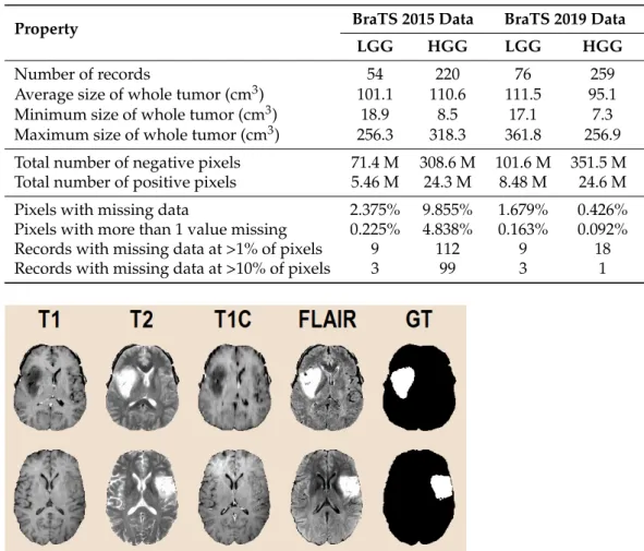
This study uses the MICCAI BraTS training data sets, both low- and high-grade glioma volumes for the years 2015 and 2019. Some main attributes of these data sets are exhibited in Table1. Only one out of these four data sets is used at a time, so in any scenario, the total numbernρof involved records varies between 54 and 259, as indicated in the first row of the table.
The records in each set have the same format. Records are multi-spectral, which means that every pixel in the volumes has four different observed intensity values (named T1, T2, T1C, and FLAIR after the weighting scheme used by the MRI device) recorded independently of each other and registered together afterwards with an automatic algo- rithm. Each volume contains 155 square shaped slices of 240×240 pixels. Pixels are isovolumetric as each of them represents brain tissues from a 1 mm3sized cubic region.
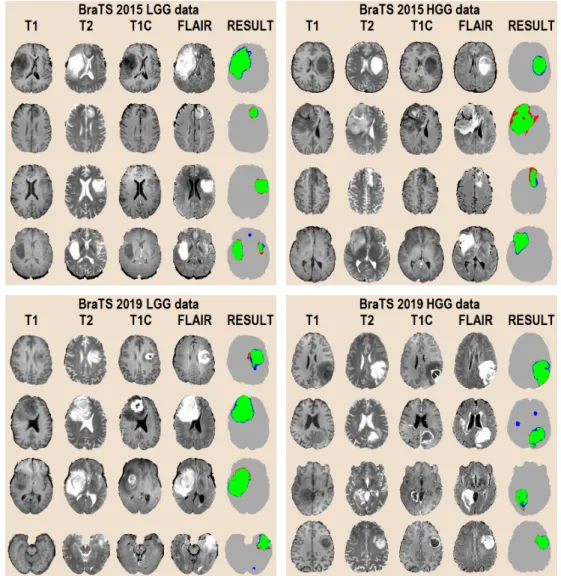
Pixels were annotated by human experts using a semi-automatic algorithm, so they have a label that can be used as the ground truth for supervised learning. Figure2shows two arbitrary slices, with all four observed data channels, and the ground truth for the whole tumor, without distinguishing tumor parts. Since the adult human brain has a volume of approximately 1500 cm3, records contain around 1.5 million pixels. Each record contains gliomas of a total size between 7 and 360 cm3. The skull was removed from all volumes so that the researchers can concentrate on classifying brain tissues only, but some of the records intentionally had missing or altered intensity values, in the amount of up to one
third of the pixels, in one of the four data channels. An overview of these cases is also reported in Table1.
Table 1.The main properties of the MRI data sets involved in this study.
Property BraTS 2015 Data BraTS 2019 Data
LGG HGG LGG HGG
Number of records 54 220 76 259
Average size of whole tumor (cm3) 101.1 110.6 111.5 95.1
Minimum size of whole tumor (cm3) 18.9 8.5 17.1 7.3
Maximum size of whole tumor (cm3) 256.3 318.3 361.8 256.9 Total number of negative pixels 71.4 M 308.6 M 101.6 M 351.5 M Total number of positive pixels 5.46 M 24.3 M 8.48 M 24.6 M
Pixels with missing data 2.375% 9.855% 1.679% 0.426%
Pixels with more than 1 value missing 0.225% 4.838% 0.163% 0.092%
Records with missing data at >1% of pixels 9 112 9 18 Records with missing data at >10% of pixels 3 99 3 1
Figure 2.Input data after pre-processing (T1 , T1C , T2, FLAIR) and the human expert made ground truth (GT) for the whole tumor segmentation problem.
Intensity non-uniformity (INU) is a low-frequency noise with possibly high magni- tude [45,46]. In the early years of the BraTS challenges, INU was filtered from the training and test data provided by the organizers. However, in later data sets, this facility is not granted. This is why we employed the method of Tustison et al. [47] to check the presence of INU and to eliminate it when necessary.
There are several non-brain pixels in the volume of any record, a fact indicated by zero intensity on all four data channels. Furthermore, there are some brain pixels in most volumes for which not all four nonzero intensity values exist; some of them are missing.
Our first option to fill missing values is to replace them with the average computed from the 3×3×3 cubic neighborhood of the pixel, if there are any pixels in the neighborhood with valid nonzero intensity. Otherwise, the missing value becomesγ0.5after pre-processing, which is the middle value of the target intensity interval; see the definition in Section2.3.
2.3. Histogram Normalization
Although very popular among medical imaging devices due to its high contrast and relatively good resolution, MRI has a serious drawback: the numerical values it produces do not directly reflect the observed tissues. The correct interpretation of the MRI data requires adapting the numerical values to the context, which is usually accomplished via a histogram normalization or standardization. Figure3gives a convincing example why the normalization of histograms is necessary. This is what we get if we represent on the same
scale the observed intensities from twenty different MRI records, extracted from the same data channel (T1). In some cases, the spectra of intensities from two different records do not even overlap. There is no classification method that could deal with such intensities without transforming the input data before classification.
Figure 3.Slice Number 100 from the T1 volume of twenty MRI records from the BraTS 2015 LGG data, without histogram normalization. These pixel intensities are obviously not suitable for any supervised classification.
Several algorithms exist in the literature for this purpose (e.g., [48–50]), more and more sophisticated histogram matching techniques, which unfortunately are not designed for records containing focal lesions. These lesions may grow to 20–30% of the brain volume, which strongly distorts the histogram in MRI channels of any weighting. The most popular histogram normalization method proposed by Nyúl et al. [48] works in batch mode, registering the histogram of each record to the same template. Modifying all histograms to look similar, no matter whether they contain tumor or not, is likely to obstruct the accurate segmentation. The method of Nyúl et al. uses some predefined landmark points (percentiles) to accomplish a two-step transformation of intensities. Many recent works [51–55] reported using this method, omitting any information on the employed landmark points. Pinto et al. [12] and Soltaninejad et al. [13] used 10 and 12 landmark points, respectively. Alternately, Tustison et al. [11] deployed a simple linear transformation of intensities, because it gives slightly better accuracy, but they did not specify any details.
This finding was confirmed later in a comparative study by Gy˝orfi et al. [56], which also showed that if we stick to the above-mentioned popular method of Nyúl et al., it provides better segmentation of focal lesions when used with a smaller number (no more than five) of landmark points, or in other words, with less restrictions.
Our histogram normalization method relies on a context dependent linear transform.
The main goal of this transform is to map the pixel intensities from each data channel of a volume independently of each other onto a target interval[α,β]in such a way that target intensities satisfy some not very restrictive criteria. The inner values of the target interval can be written asγλ = α(1−λ) +βλ, with 0 ≤ λ ≤ 1. Obviously,α = γ0andβ = γ1. To compute the two coefficients of the linear transform applied to the intensities from a certain data channel of any record, first we identify the 25th-percentile and 75th-percentile value of the original intensities and denote them by p25andp75, respectively. Then, we define theI→aI+btransform of the intensities in such a way thatp25is mapped onto γ0.4andp75becomesγ0.6. This assumption leads to the coefficients:
a= γ0.6−γ0.4
p75−p25 andb= γ0.4p75−γ0.6p25
p75−p25 . (1)
Finally, all pixel intensities from the given data channel of the current MRI record are transformed according to the formula:
Iˆ=min{max{α,aI+b},β} , (2) using the valuesaandbgiven by Equation (1), whereIand ˆIstand for the original and transformed intensities, respectively. This formula assures that the transformed intensities are always situated within the target interval[α,β].
2.4. Feature Generation
Feature generation is a key component of the procedure, because the four observed features, namely the T1, T2, T1C, and FLAIR intensities provided by the MRI device, do not contain all the possible discriminative information that can be employed to distinguish tumor pixels from normal ones. A major motivation for feature generation represents the fact that the automated registration algorithm used by the BraTS experts to align the four data channels never performs a perfect job, so for an arbitrary cubic millimeter of brain tissues, represented by the pixel situated at coordinates(x,y,z)in volume T1, the corresponding information in the other volumes is not in the same place, but somewhere in the close neighborhood of(x,y,z). A further motivation consists of the usual property of image data that neighbor pixels correlate with each other.
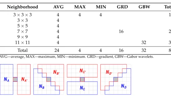
All four MRI data channels equally contribute to the feature generation process. Ob- served features are treated independently of each other: 20 computed features are extracted from each of them. The inventory of extracted features is presented in Table2. Minimum, maximum, and average values are extracted in such a way that only the brain pixels are taken into consideration from the neighborhoods indicated in the table. The computation of the gradient features involves the masks presented in Figure4. The current pixel is part of all masks to avoid division by zero in Equation (3). The 16 gradient features of an arbitrary pixelpare computed with the formula:
g(c)m (p) =γ0.5+kg
q∈Nm∑(p)∩ΩIq(c)
|Nm(p)∩Ω| −
q∈Nm∑0(p)∩ΩIq(c)
|Nm0(p)∩Ω|
, (3)
followed byg(c)m (p) ← min{max{α,gm(c)(p)},β}to stay within the target interval[α,β], wherec ∈ {T1, T2, T1C, FLAIR}is one of the four data channels,m∈ {A,B,C,D}is the index of the current gradient mask,Ωstands for the set of all brain pixels in the volume, γ0.5is the middle of the target interval of intensities,kgis a globally constant scaling factor, and|Q|represents the cardinality of any set denoted byQ.
Table 2.Inventory of computed features. Observed data channels were equally involved. Together with the four observed features, the total feature count isnϕ=84.
Neighborhood AVG MAX MIN GRD GBW Total
3×3×3 4 4 4 12
3×3 4 4
5×5 4 4
7×7 4 16 20
9×9 4 4
11×11 4 32 36
Total 24 4 4 16 32 80
AVG—average, MAX—maximum, MIN—minimum. GRD—gradient, GBW—Gabor wavelets.
Figure 4.Neighborhoods used for the extraction of gradient features, with respect to the current pixel indicated by grey color.
2.5. Multi-Atlas-Based Data Enhancement
In image segmentation, atlases are usually used as approximative maps of the objects that should be present in the image in the normal case. Atlases are usually established based on prior measurements. The image data before the current segmentation is registered to the atlas, and the current segmentation outcome is fused with the atlas to obtain a final, atlas assisted segmentation result.
In this study, we use atlases in a different manner. We build a spatial atlas for each feature using the training records, which contains the local average and standard deviation of the intensity values taken from normal pixels only. Of coarse, the training records need to be registered to each other so that we can build consistent atlases. These atlases are then used to refine the feature values in both the training and test records, before proceeding to the ensemble learning-based classification.
First of all, it is important to define the spatial resolution of atlases, which depends on a single parameter denoted byS. Each atlas is a discrete spatial array defined onS3, where S ={−S,−S+1, . . . 0 . . . ,S−1,S}. Within the atlas array, the neighborhood of atlas point
ˆ
πhaving the coordinates(x, ˆˆ y, ˆz)is defined as:
Cδ(πˆ) ={(α, ˆˆ β, ˆγ)∈ S3,|αˆ−xˆ| ≤δ ∧ |βˆ−yˆ| ≤δ ∧ |γˆ−zˆ| ≤δ} , (4) whereδis a small positive integer, typically one ore two, which determines the size of the neighborhood.
The mathematical description of the atlas building process requires the introduction of several notations. LetMstand for the set of all MRI records of the chosen data set, whileM(T)andM(E)represent the current set of training and evaluation (or test) records, respectively. Obviously,M=M(T)∪ M(E), andM(T)∩ M(E)=Φ. LetMibe the record with indexi, belonging to eitherM(T)orM(E)in a certain scenario. The set of pixels belonging to recordMi is denoted byΩi, for anyi = 1 . . .nρ. The set of all pixels from all MRI records isΩ=Sni=1ρ Ωi. Any pixelπ ∈Ωhas a feature vector withnϕelements.
For any pixelπ, the value of the feature with index ϕ ∈ {1 . . .nϕ}is denoted by Iπ(ϕ). Further, letΓ(ν)andΓ(τ)be the set of negative and positive pixels, respectively, as indicated by the ground truth. Obviously,Ω=Γ(ν)∪Γ(τ), andΓ(ν)∩Γ(τ)=Φ.
A rigid registration is defined in the following, so that we can map all volumes onto the atlas. For each recordMi (i = 1 . . .nρ), a function fi : Ωi → S3is needed that maps the pixels onto the atlas, to find the corresponding atlas position for all brain pixels.
These functions map the gravity center of each brain to the atlas origin, and the standard deviations of the x,y, andzcoordinates are all transformed to S/ξ, where ξ = 2.5 is a predefined constant. From the pixel coordinates, we compute averages and standard deviations as follows:
µ(i)x = |Ω1
i| ∑
π∈Ωi
xπ
µ(i)y = |Ω1i| ∑
π∈Ωi
yπ
µ(i)z = |Ω1
i| ∑
π∈Ωi
zπ
, (5)
and then:
σx(i)=
s
|Ωi1|−1 ∑
π∈Ωi
xπ−µ(i)x
2
σy(i)= s
|Ωi1|−1 ∑
π∈Ωi
yπ−µ(i)y
2
σz(i)= s
|Ωi1|−1 ∑
π∈Ωi
zπ−µ(i)z
2
, (6)
wherexπ,yπ, andzπare the coordinates of pixelπin the brain volume. The formula of the mapping fiis:
fi(π) =
*S xπ−µ(xi)
ξσx(i)
+ ,
*S yπ−µ(yi)
ξσy(i)
+ ,
*S zπ−µ(zi)
ξσz(i)
+!
, (7)
whereh·istands for the operation of rounding a floating point variable to the closest integer.
For any feature with indexϕ∈ {1 . . .nϕ}, the atlas function has the formAϕ:S3→ R3, which for any atlas point ˆπ∈ S3is defined as:
Aϕ(πˆ) =µˆ(ϕ)πˆ , ˆσπ(ϕ)ˆ , ˆνπ(ϕ)ˆ
, (8)
where the components ˆµ(ϕ)πˆ , ˆσπ(ϕ)ˆ , and ˆνπ(ϕ)ˆ are established with the following formulas:
ˆ
ν(ϕ)πˆ = ∑
Mi∈M(T)
|Ψ(i, ˆπ)|
ˆ
µ(ϕ)πˆ =νˆπ(ϕ)ˆ −1
Mi∈M∑ (T) ∑
π∈Ψi(π)ˆ Iπ(ϕ)
!
σˆπ(ϕ)ˆ = v u u t
νˆπ(ϕ)ˆ −1−1 ∑
Mi∈M(T)
π∈Ψ∑i(π)ˆ
Iπ(ϕ)−µˆ(ϕ)πˆ 2
!
(9)
where:
Ψi(πˆ) =nπ∈Ωi∩Γ(ν),fi(π)∈ Cδ(πˆ)o . (10) The feature values of each pixelπ∈Ωi(i=1 . . .nρ), no matter whetherπbelongs to a record of the training or test data, are updated with the following formula:
eIπ(ϕ)←min
max
α,
* µ+σ
Iπ(ϕ)−µˆ(ϕ)fi(π) ˆ σ(ϕ)f
i(π)
+
,β
, (11)
where parametersµandσrepresent the target average and standard deviation, respectively, and their recommended values are:
µ=γ0.5 = (α+β)/2
σ= (β−α)/10 . (12)
Algorithm1summarizes the construction and usage of the atlas. The updated intensity values compose the pre-processed data denoted byP2in Figure1. BothP1andP2follow the very same classification and post-processing steps.
2.6. Ensemble Learning
The total number ofnρrecords is randomly separated into six equal or almost equal groups. Any of these groups can serve as test data, while the other five groups are used to train the decision making ensemble. The ensembles consist of binary decision trees, whose main properties are listed in the following:
1. The size of the ensemble is defined by the number of trees, set tonT = 125 based on intermediary tests performed on the out-of-bag (OOB) data, which are the set of feature vectors from the training data that are never selected for training the trees of a given ensemble.
2. The training data size, represented by the number of randomly selected feature vectors used to train each tree, and denoted bynF, is chosen to vary between 100 thousand and one million in four steps:nF ∈ {100k, 200k, 500k, 1000k}. These four values are
used during the experimental evaluation of the proposed method to establish its effect on the segmentation accuracy and efficiency.
3. The selection of feature vectors for training the decision trees is not totally random.
The balance of positive and negative feature vectors in the training set of each BDT is defined by the rate of negativesp−and rate of positivesp+. For the LGG and HGG data sets,p−=93% andp−=91% are used, respectively, values set according to the findings of intermediary tests performed on OOB data.
4. Trees are trained using an entropy-based rule, without limiting their depth, so that they can provide perfect separation of feature vectors representing pixels belonging to tumors and normal tissues. The trees of the ensemble have their maximum depth ranging between 25 and 45, depending onnFand the random training data itself.
Algorithm 1:Build the atlas functionAϕfor each featureϕ=1 . . .nϕ, and apply it to all feature data.
Data:Set of MRI records involved in the studyM, its set of pixelsΩ, each pixel with 4 observed andnϕ−4 computed features.
Data:ParametersSandδ
Result:Atlas functionsAϕ,ϕ=1 . . .nϕ
Result:Updated intensities in all records ofM
Define the set of training and test records,M(T)andM(E), respectively.
for eachMi∈ Mdo
Compute the mapping function fi(π)for every pixelπ∈Ωiusing Equations (5)–(7).
end
forϕ=1 . . .nϕdo
Compute the atlas functionAϕ(πˆ)for every discrete point ˆπ∈ S3having ˆ
νπ(ϕ)ˆ >1, using Equations (8)–(10).
for eachMi∈ Mdo for eachπ∈Ωido
Update the value of featureϕof pixelπusing the formula given in Equation (11).
end end end
When all trees of the ensemble are trained, they can be used to obtain the prediction for the feature vectors from the test data records. Each pixel from the test records receives nTvotes, one from each BDT. The decision of the ensemble is established by the majority rule, and that gives a label to each test pixel. However, these are intermediary labels only, as they undergo a twofold post-processing. The intermediary labels received by test pixels compose theS1andS2segmentation results indicated in Figure1.
2.7. Random Forest-Based Post-Processing
The first post-processing step reevaluates the initial label received by each pixel of the test data records. The decision is made by a random forest classifier that relies on morphological features. The details of this post-processing step are listed in the following:
1. The RF is trained to separate positive and negative pixels using six features extracted from the intermediary labels produced by the BDT ensemble. Let us considerK=5 concentric cubic neighborhoods of the current pixel, denoted byNk (k = 1 . . .K), each having the size(2k+1)×(2k+1)×(2k+1). Inside the neighborhoodNkof the current pixel, the count of brain pixelsnkand the count of positive intermediary labeled brain pixelsn+k is extracted. The ratioρk =n+k/nkis called the rate of positives within neighborhoodNk. The feature vector has the form(ρ1,ρ2, . . .ρK,η), whereηis
the normalized value of the number of complete neighborhoods of the current pixel, determined as:
η= 1 K
∑
K k=1δ
nk,(2k+1)3 , (13) where:
δ(u,v) =
1 ifu=v
0 otherwise . (14)
2. To assure that testing runs on data never seen by the training process, pixels from HGG tumor volumes are used to train the random forest applied in the segmentation of LGG tumor volumes, and vice versa. Each forest is trained using the feature vectors of 107randomly selected voxels, whose feature values fulfil∑Kk=1ρk>0.
3. Pixels whose features satisfy∑Kk=1ρk =0 are declared negatives by default; they are not used for training the RF and are not tested with the RF either.
4. The number of trees in the RF is set to 100, while the maximum allowed depth of the trees is eight.
The result of this post-processing step can be seen in Figure1, represented by segmen- tation resultsS01andS02.
2.8. Structural Post-Processing
The structural post-processing handles only pixels that are labeled positive in segmen- tation resultsS01andS02; consequently, it has the option to approve or discard the current positive labels. As a first operation, it searches for contiguous spatial regions formed by positive pixels within the volume using a region growing algorithm. Contiguous regions of positive labeled pixels with a cardinality below 100 are discarded, because such small lesions cannot be reliably declared gliomas. Larger lesions are subject to shape-based validation. For this purpose, the coordinates of all positive pixels belonging to the cur- rent contiguous region undergo a principal component analysis (PCA), which establishes the three main axes determined by the three eigenvectors and the corresponding radii represented by the square root of the three eigenvalues provided by PCA. We denote by λ1>λ2>λ3the three eigenvalues in decreasing order. Lesions having the third radius below a predefined threshold (√
λ3< 2) are discarded, as they are considered unlikely shapes for a glioma. All those detected lesions that are not discarded by the criteria pre- sented above are finally declared gliomas, and all their pixels receive final positive labels.
This is the final solution denoted byS100andS002in Figure1.
2.9. Evaluation Criteria
The whole set of pixels of the MRI record with indexiisΩi, which is separated by the ground truth into two disjoint sets: Γ(π)i andΓ(ν)i , the set of positive and negative pixels, respectively. The final segmentation result provides another separation ofΩiinto two disjoint sets denoted byΛ(π)i andΛ(ν)i , which represent the positive and negative pixels, respectively, according to the final decision (labeling) of the proposed procedure.
Statistical accuracy indicators reflect in different ways how much the subsetsΓ(π)i andΛ(π)i and their complementary subsetsΓ(ν)i andΛ(ν)i overlap. The most important accuracy markers obtained for any record with indexi(i=1 . . .nρ) are:
1. Dice similarity coefficient (DSC) or Dice score:
DSCi = 2× |Γ(π)i ∩Λ(π)i |
|Γ(π)i |+|Λ(π)i | , (15)
2. Sensitivity or true positive rate (TPR):
TPRi= |Γ(π)i ∩Λi(π)|
|Γ(π)i | , (16)
3. Specificity or true negative rate (TNR):
TNRi= |Γ(ν)i ∩Λ(ν)i |
|Γ(ν)i | , (17)
4. Positive predictive value:
PPVi = |Γ(π)i ∩Λ(π)i |
|Λ(π)i | , (18)
5. Accuracy or rate of correct decisions (ACC):
ACCi = |Γ(π)i ∩Λ(π)i |+|Γ(ν)i ∩Λ(ν)i |
|Γ(π)i |+|Γ(ν)i | . (19) To characterize the global accuracy, we may compute the average values of the above- defined indicators over a whole set of MRI records. We denote them by DSC, TPR, TNR, PPV, and ACC. The average Dice similarity coefficient is given by the formula:
DSC= n1
ρ nρ
i=1
∑
DSCi . (20)
The average values of other accuracy indicators are computed with analogous formulas.
The overall Dice similarity coefficient (]DSC) is a single Dice score extracted from the set of all pixels fromΩ, given by the formula:
DSC]= 2×
nρ
S
i=1Γ(π)i ∩ nSρ
i=1Λ(π)i
nρ
S i=1Γ(π)i
+
nρ
S i=1Λ(π)i
. (21)
All accuracy indicators are defined in the[0, 1]interval. Perfect segmentation sets all indicators to the maximum value of 1.
3. Results
The proposed brain tumor segmentation procedure was experimentally evaluated in various scenarios. Tests were performed using four different data sets: the LGG and HGG records separately from the BraTS 2015 training data set and, similarly, the LGG and HGG records separately from BraTS 2019 training data set. Detailed information on these data sets is given in Table1. The whole segmentation process was the same for all four data sets, the one indicated in Figure1.
All records of these four data sets underwent the mandatory pre-processing steps, namely the histogram normalization and feature generation, resulting in pre-processed data denoted byP1. At this point, the records were randomly separated into six equal or almost equal groups, which took turns serving as the test data. An atlas was built using the training data only, namely the records from the other five groups. The atlas was then used to extract enhanced feature values for all records, resulting in pre-processed data denoted byP2. During the whole processing, there were six different such sets denoted byP2, one for the testing of each group.
Preprocessed data setsP1andP2underwent the ensemble learning process separately, so that we could evaluate the benefits of the atlas-based pre-processing. All ensembles involved in this study consisted ofnT = 125 binary decision trees, but there were four variants for each data set, in terms of training data size. Each tree of an ensemble was trained to separatenFfeature vectors,nFranging from 100 thousand to on million, as indi- cated in Section2.6. The intermediary segmentation obtained at the ensemble output is denoted byS1orS2, depending on the use of the atlas during pre-processing. The labels of pixels inS1orS2were treated with two post-processing steps described in detail in Sections2.7and2.8, reaching the final segmentation denoted byS100orS002. Theoretically, all six segmentation resultsS1,S2,S01,S20,S001, andS002 can be equally evaluated with the statistical measures presented in Section2.9. The main result is represented by the final outcome of the segmentation: S001 for the data that are not pre-processed with the atlas andS200for the data with atlas-based enhancement.
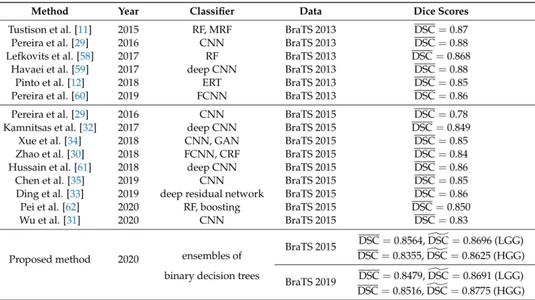
Table3presents the average (DSC) and overall (DSC) values of the Dice similarity] coefficients obtained for various data sets and training data sizes, at four different phases of the segmentation process. A larger training data size always led to better accuracy: both the average and overall value rose by 0.5–0.8% if the training data size changed from 100k to 1000k. If we consider segmentation accuracy the only important quality marker, then it is worth using the largest training data size. The use of the atlas was beneficial in all scenarios, but there were large differences in the strength of this effect: at the ensemble output, the difference was between 0.3% and 2%, while at the final segmentation, it was between 0.2% and 1%. The difference between the average and overall values in the same scenario usually ranged between 2% and 3%. This was caused by the distribution of the Dice similarity coefficients obtained for individual MRI records. The obtained Dice scores, having most averages between 0.85 and 0.86 and overall values ranging between 0.86 and 0.88, were quite competitive.
Table 3.Average and overall Dice similarity coefficients obtained for various data sets and training data sizes, with and without atlas-based data enhancement at pre-processing.
Segmentation Train BraTS 2015 LGG BraTS 2015 HGG BraTS 2019 LGG BraTS 2019 HGG
Result Data Size DSC DSC] DSC DSC] DSC DSC] DSC DSC]
ensemble
(S1)
100k 0.7904 0.8217 0.7827 0.8248 0.7693 0.8065 0.8232 0.8560
output 200k 0.7928 0.8239 0.7858 0.8267 0.7748 0.8113 0.8264 0.8578
without 500k 0.7961 0.8266 0.7903 0.8290 0.7795 0.8154 0.8300 0.8602
atlas 1000k 0.7980 0.8284 0.7935 0.8310 0.7828 0.8185 0.8324 0.8619
final
(S001)
100k 0.8470 0.8618 0.8217 0.8524 0.8266 0.8495 0.8421 0.8679
result 200k 0.8490 0.8635 0.8241 0.8540 0.8309 0.8531 0.8436 0.8692
without 500k 0.8515 0.8657 0.8276 0.8557 0.8347 0.8565 0.8452 0.8707
atlas 1000k 0.8536 0.8674 0.8300 0.8571 0.8378 0.8591 0.8464 0.8717
ensemble
(S2)
100k 0.8040 0.8316 0.7943 0.8279 0.8015 0.8307 0.8259 0.8602
output 200k 0.8063 0.8336 0.7963 0.8301 0.8047 0.8337 0.8281 0.8626
with 500k 0.8089 0.8359 0.7990 0.8334 0.8074 0.8367 0.8307 0.8654
atlas 1000k 0.8107 0.8375 0.8013 0.8357 0.8091 0.8386 0.8326 0.8675
final
(S002)
100k 0.8503 0.8646 0.8299 0.8573 0.8412 0.8624 0.8464 0.8738
result 200k 0.8519 0.8662 0.8317 0.8588 0.8442 0.8652 0.8485 0.8751
with 500k 0.8547 0.8683 0.8337 0.8610 0.8470 0.8681 0.8504 0.8766
atlas 1000k 0.8564 0.8696 0.8355 0.8625 0.8479 0.8691 0.8516 0.8775
Tables4–7exhibit the average sensitivity, positive predictive value, specificity, and cor- rect decision rate (accuracy) values, respectively, obtained for different data sets and various training data sizes. Not all these indicators increased together with the training data size, but the rate of correct decisions did, showing that it is worth using a larger amount of
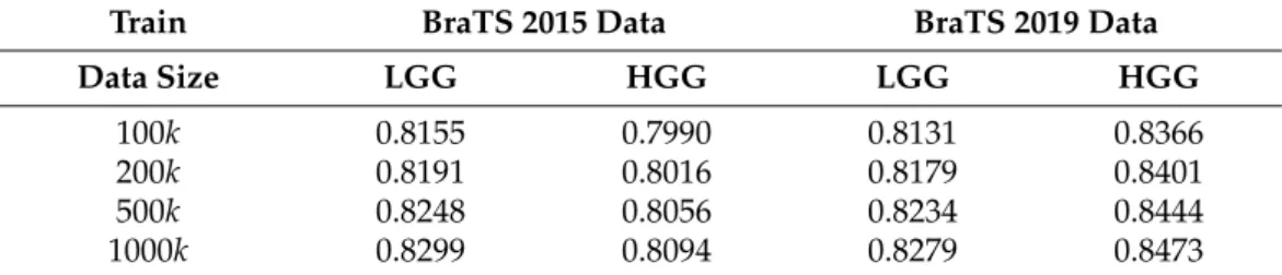
training data to achieve better segmentation quality. Sensitivity values were in the range 0.8–0.85, while positive predictive values around 0.9, which indicate a fine recognition of true tumor pixels. Specificity rates were well above 0.99, which is highly important because it grants a reduced number of false positives. The average rate of correct decisions, with its values mostly above 0.98, indicates that one out of fifty or sixty pixels was misclassified by the proposed segmentation procedure. All values from Tables4–7reflect the evalu- ation of the final segmentation outcomes denoted byS002, obtained from atlas enhanced pre-processed data.
Table 4.Average sensitivity values (TPR)—final result with atlas(S200).
Train BraTS 2015 Data BraTS 2019 Data
Data Size LGG HGG LGG HGG
100k 0.8155 0.7990 0.8131 0.8366
200k 0.8191 0.8016 0.8179 0.8401
500k 0.8248 0.8056 0.8234 0.8444
1000k 0.8299 0.8094 0.8279 0.8473
Table 5.Average positive predictive values (PPV)—final result with atlas(S002).
Train BraTS 2015 Data BraTS 2019 Data
Data Size LGG HGG LGG HGG
100k 0.9071 0.8935 0.9055 0.8888
200k 0.9064 0.8936 0.9046 0.8878
500k 0.9043 0.8923 0.9032 0.8857
1000k 0.9019 0.8909 0.8986 0.8842
Table 6.Average specificity values (TNR)—final result with atlas(S002).
Train BraTS 2015 Data BraTS 2019 Data
Data Size LGG HGG LGG HGG
100k 0.9936 0.9913 0.9933 0.9923
200k 0.9935 0.9913 0.9932 0.9922
500k 0.9933 0.9912 0.9931 0.9920
1000k 0.9931 0.9910 0.9927 0.9919
Table 7.Average accuracy values (ACC)—final result with atlas(S002).
Train BraTS 2015 Data BraTS 2019 Data
Data Size LGG HGG LGG HGG
100k 0.9812 0.9792 0.9796 0.9837
200k 0.9814 0.9794 0.9799 0.9838
500k 0.9816 0.9796 0.9803 0.9840
1000k 0.9817 0.9797 0.9803 0.9840
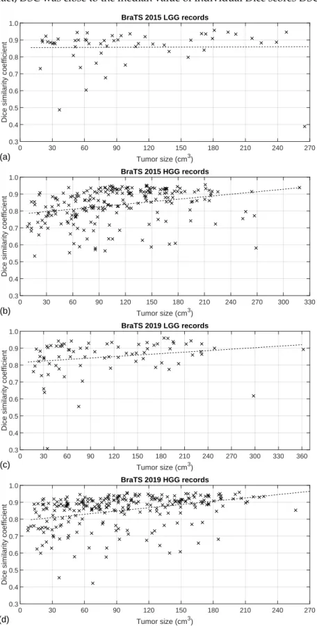
Figure5exhibits the Dice similarity coefficients obtained for individual MRI records (DSCi, fori=1 . . .nρ) plotted against the true size of the tumor according to the ground truth. Each cross represents one of the MRI records, while the dashed lines indicate the linear trend of the DSCivalues identified with linear regression. As was expected, the linear trends indicate better segmentation accuracy for larger tumors. It is also visible that for most tumors, we achieved a Dice score above 0.8, and there were some records below that limit where the Dice scores could be very low. This is mostly because not all records in the BraTS data have the same image quality; some of them even contain artificially created obstacles. This distribution of the DSCi values is also the reason why the overall Dice
similarity value was higher than the average (DSC]>DSC) in case of all four data sets. In fact,DSC was close to the median value of individual Dice scores DSC] i,i=1 . . .nρ.
Tumor size (cm3)
0 30 60 90 120 150 180 210 240 270
Dice similarity coefficient
0.3 0.4 0.5 0.6 0.7 0.8 0.9
1.0 BraTS 2015 LGG records
(a)
Tumor size (cm3)
0 30 60 90 120 150 180 210 240 270 300 330
Dice similarity coefficient
0.3 0.4 0.5 0.6 0.7 0.8 0.9
1.0 BraTS 2015 HGG records
(b)
Tumor size (cm3)
0 30 60 90 120 150 180 210 240 270 300 330 360
Dice similarity coefficient
0.3 0.4 0.5 0.6 0.7 0.8 0.9
1.0 BraTS 2019 LGG records
(c)
Tumor size (cm3)
0 30 60 90 120 150 180 210 240 270
Dice similarity coefficient
0.3 0.4 0.5 0.6 0.7 0.8 0.9
1.0 BraTS 2019 HGG records
(d)
Figure 5.Individual Dice scores plotted against the true size of the tumor: (a) 54 records of BraTS 2015 LGG data; (b) 220 records of BraTS 2015 HGG data; (c) 76 records of BraTS 2019 LGG data; (d) 259 records of BraTS 2019 HGG data.
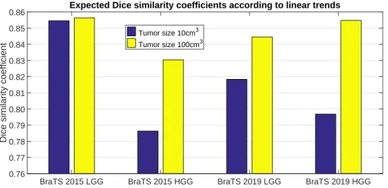
Figure6presents the Dice similarity scores we may expect for a 10 cm3and a 100 cm3


![Table 3 presents the average (DSC) and overall ( DSC) values of the Dice similarity ] coefficients obtained for various data sets and training data sizes, at four different phases of the segmentation process](https://thumb-eu.123doks.com/thumbv2/9dokorg/750130.31563/14.892.53.856.686.1059/presents-average-similarity-coefficients-obtained-training-different-segmentation.webp)