Handling of tire pressure variation in autonomous vehicles: an integrated estimation and control design approach
Tam´as Heged˝us, D´aniel F´enyes, Bal´azs N´emeth and P´eter G´asp´ar
Abstract— Tire pressure has a high impact on the tire-road contact because it influences the characteristics of the tire forces. During the maneuvering of the vehicle the pressures of the tires may decrease over time, which results in performance degradation or the loss of controllability. This paper proposes a novel integration of tire pressure estimation and path- following control design based on machine learning and Linear Parameter-Varying (LPV) methods. In the estimation process the vehicle dynamic signals, which are available from the conventional on-board sensors, are fused. The values of the estimated tire pressures are incorporated in the LPV control as scheduling variables. The results of the control system are the steering and the differential drive interventions on the vehicle. The effectiveness of the method is illustrated through comprehensive simulation scenarios through the CarMaker simulation enviroment.
I. INTRODUCTION AND MOTIVATION
Nowadays, one of the main goals of the automotive industry is to develop more automated and self-driving, autonomous vehicles, which are more reliable and provide safer ride for the passengers. This task includes numerous challenges which manufacturers must meet. Besides these challenges, the reduction of vehicle production and operation costs is expected. This reduction in cost can be achieved by using fewer sensors, since some of them are expensive, such as pressure sensors or high-accuracy GPS. Since the vehicles are already equipped with various low-cost sensors, e.g. accelerometers, gyroscopes, the fusion of these devices can be used to provide continuous information about the vehicle and its environment. An advantage of this technology is that hidden indirect information about unmeasured vehicle parameters through appropriate fusions might be revealed.
T. Heged˝us is with Department of Control for Transportation and Vehicle Systems, Budapest University of Technology and Eco- nomics, M˝uegyetem rkp. 3, H-1111 Budapest, Hungary. E-mail: hege- dus.tamas@mail.bme.hu
D. F´enyes, B. N´emeth, P. G´asp´ar are with Systems and Control Laboratory, Institute for Computer Science and Control, Kende u. 13-17, H-1111 Budapest, Hungary. E-mail:
[daniel.fenyes;balazs.nemeth;peter.gaspar]@sztaki.mta.hu
The work was supported by the research program titled ”Exploring the Mathematical Foundations of Artificial Intelligence (2018-1.2.1-NKP- 00008).
The research was supported by the Hungarian Government and co- financed by the European Social Fund through the project ”Talent manage- ment in autonomous vehicle control technologies” (EFOP-3.6.3-VEKOP- 16-2017-00001).
The work of B. N´emeth was partially supported by the J´anos Bolyai Re- search Scholarship of the Hungarian Academy of Sciences and the UNKP- 19-4 New National Excellence Program of the Ministry for Innovation and Technology. The works of D. F´enyes and T. Heged˝us were partially supported by the UNKP-19-3 New National Excellence Program of the Ministry for Innovation and Technology.
Further application possibilities are that redundancy in sen- sors can be eliminated or they can be used to detect sensor failures.
The estimation of tire pressure is a promising field of vehicle control, in which the special tire pressure sensor can be eliminated through data fusion. Although the special tire pressure sensors may have good performance in the precise estimation of the pressure (see e.g. [1]), the solution has some drawbacks. It increases the cost of the vehicle and in case of a wheel change it can require a calibration process.
Moreover, some sensors require an external energy source.
Although there are energy-harvesting technologies to avoid the necessity of the batteries [2], [3], these sensors require improved production methods. Thus, the fusion of the vehicle dynamic signals is an alternative solution in the estimation problem of the tire pressure. Through the increased amount of information in the automated vehicles big data analysis provides a new impulse of research.
In the field of tire pressure estimation various methods have been presented, see e.g. [4], [5]. There are further results which address tire pressure loss as a controllability problem.
When a tire starts losing its pressure, the maneuverability of the vehicle deteriorates as well since the maximum value of the realizable lateral force depends strongly on the pressure.
Paper [6] focuses on this control problem, using aH∞-based control system. This control algorithm is able to guarantee the robustness of the motion of the vehicle in the presence of pressure loss. Another solution is presented in [7], in which the authors use a flatness-based Model Predictive Controller to ensure the stability of the vehicle when a tire blow-out occurs. The results show that tire pressure has a high impact in the dynamics and control of the vehicle. The improvement of the control performance requires an appropriate estimation of tire pressure, which means that the estimation and the control methods are in strong relationship. However, in general the papers handle the problem separately.
The contribution of the paper is to propose an intercon- nection of the tire pressure estimation and the vehicle control methods. The estimation is based on a machine learning process, which is based on the collected big data of the vehicle signals. The result of the estimation is incorporated in the vehicle control design through the Linear Parameter- Varying (LPV) control design theory, in which the tire pressure is addressed as a scheduling variable. The outputs of the proposed estimator-controller structure are the steering angles on the front wheel and the torque of the differential driving. Through the resulting control inputs the motion of the vehicle at the loss of pressure can be stabilized and a 2020 American Control Conference
Denver, CO, USA, July 1-3, 2020
good vehicle maneuvering performance can be achieved.
The structure of the paper is as follows: Section II pro- poses the method of data collection and analysis. It also presents the applications and the results of the applied deep- learning algorithm for pressure estimation purposes. The LPV control design method with the incorporation of the estimation results is presented in Section III. Moreover, Section IV shows results of simulation scenarios. Finally, the contributions of the paper and the further challenges are summarized in Section V.
II. DESIGN OF VEHICLE PRESSURE ESTIMATOR THROUGH MACHINE LEARNING
The purpose of this section is to present the design of the tire pressure estimation method using various measured signals, which requires the collection of the training data, training and test processes of the neural network.
A. Acquisition of training data from simulations
Machine learning techniques require large amount of data to provide reliable estimation models. Therefore, numerous simulations have been performed using the high-fidelity car simulation software CarMaker. It contains the built-in Pacejka Magic Formula tire model [8], which is able to handle the variation of the tire pressure. In a simulation scenario the pressure values of the tires are constant, but they are varied between the scenarios: the maximum value of the pressure has been set at pmax = 2.5 bar, while the minimum value of the pressure has been pmin = 1.0 bar.
The step size of the pressure between the limits has been selected∆p= 0.3 bar.
During the data acquisition process the pressure values in the front left and front right tires are varied. The initial velocity of the vehicle is selected between11−15m/sand a PI controller is applied as a cruise control. The sampling time of the simulations is set atTs= 0.01s.
Several measurements are collected in the simulation scenarios, such as lateral and longitudinal velocities, steering angle, yaw rate, accelerations, wheel speeds, forces on the tires etc. Finally, over 1 million instances have been col- lected, which can be used for the learning process. After the data acquisition the data set must be filtered to eliminate the worthless scenarios. For example, the longitudinal velocity of the vehicle covers a large range, sometimes the vehicle is not able to follow the predefined path at high velocities.
These scenarios are caused by the unstable behaviour of the vehicle, which is out of the region of interest from the aspect of the estimator design.
B. Brief overview of neural network
The neural network is a member of the machine learning family. The artificial neural network is modeled after the human brain in such a manner that it is able to solve complex, nonlinear problems. The main advantage which distinguishes this technique from the conventional machine learning algorithms is its ability to deal with different kinds
of optimization tasks, such as clustering, classification, pre- diction etc. A neural network contains weights and activation functions, which are called neurons. They are grouped into layers. A network has one input and one output layers and, at least, one hidden layer. The number of the hidden layers and the type of the activation function can be chosen freely, and they are the main parameters of the neural network [9].
In this paper the neural network is trained for estimation purposes. The structure of the network consists of one input, one output and 3 hidden layers. The hidden layers contain 55-45-55 neurons. The numbers of the hidden layers and the neurons are selected by using the so-called k-fold cross validation technique [10]. Initially, this method divides the dataset into two subsets. The first subset is the training set, which used for training the network. The other subset is the test set which is used for evaluating the neural network.
Moreover, another crucial part of the network is the used ac- tivation functions. Although there exists numerous functions that can be used in the training process, the rectified linear unit (ReLU) and the log-sigmoid functions are used in this estimation problem, because they can be easily adjusted to nonlinear problems. For training the network, the Levenberg- Marquardt algorithm is used [11].
C. Evaluation of the neural networks
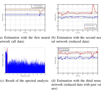
In the following, the results of the machine learning based estimation are presented through illustrations. The goal of the neural network is to estimate the pressures of the front tires separately. Various neural networks have been created using different attributes to find the best applicable estimation model. The effectiveness of the networks are compared below. During the simulations the pressures of the tires are set at1.5barand2.0bar, respectively.
In the case of the first neural network all of the collected attributes are used, see Figure 1(a) for the estimated pres- sures. Since the measurements can be influenced by noises and disturbances, a 0.2bar wide interval is determined, in which the estimation is considered to be acceptable. The dashed lines illustrate the borders of the interval. The output of the neural network is rounded to0.1. Figure 1(a) shows that the neural network provides an accurate estimation for the pressures. In the last part of the simulation the vehicle has high side-slip values, which degrade the estimation performance.
Although the first neural network has a good estimation performance, in practice not all of the collected attributes can be directly measured on the vehicle. Thus, second neural network has been trained, which has been built up using the measurements. They are available on the vehicle on-board, such as wheel speeds, accelerations, longitudinal velocity, yaw rate and the steering angle. The results of the second estimator can be seen in Figure 1(b). As the figure shows, this network provides less accurate estimation compared to the previous one, but its result is still sufficiently accurate to be used in the control system.
In order to improve the estimation, the past values of the measurements are also used in the third neural network. The
effective incorporation of the past information requires the selection of the most influential past values. Thus, a spectral analysis is performed, whose result is shown in Figure 1(c).
The examination shows that the information content of the signal is below 6Hz, which means that the time interval between two consecutive points is set atT = 1/6Hz= 0.15 s. In this manner, the most significant values can be selected and the number of the used past values can be limited.
The third neural network is learning based on the extended training set. The result of the network is shown in Figure 1(d). Although it can be seen that this network provides more fluctuating output, the peak value of error signal has decreased significantly.
0 10 20 30 40 50 60 70 80
Time (s) 0
0.5 1 1.5 2 2.5
Pressure (bar)
Front left tire Front right tire
(a) Estimation with the first neural network (all data)
0 10 20 30 40 50 60 70 80
Time (s) 0
0.5 1 1.5 2 2.5 3
Pressure (bar)
Front left tire Front right tire
(b) Estimation with the second neu- ral network (reduced data)
(c) Result of the spectral analysis
0 10 20 30 40 50 60 70 80
Time (s) 0
0.5 1 1.5 2 2.5
Pressure (bar)
Front left tire Front right tire
(d) Estimation with the third neural network (reduced data with past val- ues)
Fig. 1. Results of the tire pressure estimation with various neural networks
In Table I, the presented neural networks are compared based on statistical values. The average error is related to
TABLE I
STATISTICAL COMPARISON OF THE NEURAL NETWORKS
Tire (L/R) All data Past data Accuracy Av. error
Lef t 3 7 100% 0.00
Right 3 7 96.1% 0.0072
Lef t 7 3 90.3% 0.01522
Right 7 3 94.4% 0.00552
Lef t 7 7 83.3% 0.0554
Right 7 7 92.2% 0.01
the error of the pressure estimation, while the accuracy represents the ratio, when the estimated signal is inside of the predefined interval. As the figures have shown, the best result is given by the first network, which uses all of the attributes (100% and96.1%). However, it cannot be used in practice due to the lack of several signals in the measurement. An accurate estimation is provided by the third network, which uses the available variables and their past values. Although the accuracy of this network is lower (90.3% and94.4%), its average error is small (0.0055and0.0554), which means that the output of this network is sufficiently close to the
actual pressures of the tires. Thus, the third type of neural network is used in the control design.
III. LPV-BASED CONTROL USING THE ESTIMATED TIRE PRESSURES
In this section, the lateral control design based on a LPV method is presented for autonomous vehicles. As a novelty of the application, the results of the tire pressure estimation are used in the control system as scheduling parameters. The control system has two control inputs, such as the steering angle and the differential driving, which compensates for the loss of lateral force when the pressure of the tire decreases.
In the following, a lateral vehicle model is presented, which is the base of the LPV control design [12].
A. Modeling of the vehicle dynamics
In this paper, the single-track lateral vehicle model is used, which consists of the following equations [13]:
Iψ¨=Ff,y(αf)l1−Fr,y(αr)l2+Md (1a) mvx( ˙ψ+ ˙β) =Ff,y(αf) +Fr,y(αr) (1b)
˙
vy =vx( ˙ψ+ ˙β) (1c) whereIdenotes the yaw inertia,Fi,yare the lateral forces at the front and the rear axles,lxare the distances between the COG and the axles,αx, x∈ {f, r}are the side-slip angles of the front and rear wheelsαf =δ−β−ψlv˙1
x andαr=β−ψlv˙ 2
x, respectively,Mdis the generated torque from the differential drive,ψ˙ is the yaw-rate,β is the side-slip of the vehicle and vxandvy are the velocities of the vehicle andδdenotes the steering angle.
The pressures appear in the motion of the vehicle indi- rectly because they highly correlate to the cornering stiffness values. It can be expressed as a function of the pressures in the front left/right tiresp1,l, p1,r, see [8]:
Ff,y(p1,l, p1,r) =Ff,y,l(p1,l) +Ff,y,r(p1,r)
=Cf,y(p1,l)α+Cf,y(p1,r)α, (2) whereFf,y,l(p1,l), Ff,y,r(p1,r)are the forces on the left/right wheels. The relationship between the pressure and the cor- nering stiffness can be assumed to be linear based, as it is illustrated in Figure 2. In the example the maximum value of theCf,y in CarMaker is considered to be57000N/rad, while the minimum is 39000N/rad. Thus, the relationship (2) is transformed as
Ff,y(p1,l, p1,r) = 2Cf,y,0+Cf,y,1p1,l+Cf,y,1p1,r α
= 2 Cf,y,0+Cf,y,1p1
α, (3)
wherep1 is the average pressure of the wheels on the front axle.
The lateral vehicle model (1a) together with (3) are transformed into a state-space representation, such as:
˙
xv=Av(vx, p1)xv+Bv(vx, p1)uv. (4) The state vector xv consists of the signals xv = [ ˙ψ β vy y]T. The control inputs of the system areuv=
1 1.5 2 2.5 Pressure (bar)
3.5 4 4.5 5 5.5 6
Cornering stiffnes (N/rad)
104 Measured data Linear approximation
Fig. 2. Relationship between pressure and cornering stiffness
[δ Md], whereδdenotes the front-wheel steering angle. The signalsvx, p1 are selected as the scheduling variables of the system.
B. Modeling of the steering system
The dynamics of the steering system has a significant impact on the performances of the lateral control system.
Therefore, in the control design the model of the steering mechanism is also incorporated. It is formed as a second- order system, such as
Gs(s) = b2s2+b1s+b0
s2+a1s+a0
(5) where bi and ai are the parameters, which must be deter- mined through an identification process.
In this paper the ARX identification structure is used for the determination of the system parameters. The ARX structure is formed as [14]:
y(t) +a1y(t−1) +...+anay(t−na) = (6)
=b1u(t−1) +...+bnbu(t−nb) +e(t)
where y denotes the output of the system, which is the steering angle of the front wheels. Moreover,udenotes the input of the system, which is the angle of the steering wheel and e(t) represents the error function. The parameters can be written into a parameter vector:
σ= [a1 ... ana b1 ... bnb]T. (7) By using shift operatorq−1, two expressions are introduced:
A(q) = 1 +a1q−1+...+anaq−naandB(q) =b1q−1+...+ bnbq−nb. The transfer function of the identified system can be formed as:
G(q, σ) =B(q)
A(q) (8)
The resulting transfer function is a discrete-time system, which means that the resulting system must be transformed into a continuous form. For the transformation Ts = 0.01s sampling time and a zero-order hold element are used. The transformed continuous state-space representation can be formed using the continuous transfer function:
˙
xs=Asxs+Bsus, (9)
ys=cTsxs (10)
whereusis the angle of the steering wheel,ysis the steering angle of the front wheels,As,Bs andcTs are matrices. The state vectorxscontains the states of the steering system.
C. Design of the LPV control
The presented two state-space representations (4) and (9) are combined and written into an extended state-space representation:
˙
xe=Ae(vx, p1)xe+Be(vx, p1)ue, (11) whereue=[usMd]T andxe= [xs xv]T, the matrices are
Ae(vx, p1) =
As 02x4
Bv,1(vx, p1)CsT Av(vx, p1)
, (12a) Be(vx, p1) =
Bs 02x1
04x1 Bv,2(vx, p1)
, (12b)
whereBv,i(vx, p1)denotes the ithcolumn ofBv(vx, p1).
The control system is responsible for the tracking of the predefined trajectory and for the minimization of the control interventions. Therefore, the following four performances are defined.
1. Minimization of the yaw-rate error: The tracking of the road requires the reduction of the error between reference ψ˙ref and the measured yaw rate ψ˙ in order to achieve accurate and smooth tracking:
z1= ˙ψref −ψ,˙ |z1| →min, (13) whereyref is considered to be given.
2.Minimization of the lateral error: In order to achieve good tracking performance, the control system must minimize the lateral error between the road yref and the lateral position of the vehicley :
z2=yref −y, |z2| →min. (14) 3. Minimization of the steering angle: The control system must minimize the steering interventions to reduce energy consumption and to address the physical limits of the steering actuator, which means the minimization of the steering angle is formed as a performance
z3=δ, |z3| →min. (15) 4.Minimization of the differential drive: Similarly to the third performance, the controller must minimize the differential torque as well as the steering angle
z4=Md, |z4| →min. (16) The performances are summarized in the vector z = z1 z2 z3 z4T
, which leads to the performance equa- tion
z=C1xe+D11r+D12ue, (17) whereC1, D11, D12 are matrices and r contains the signal yref.
In the LPV control design, the presented extended state- space model (11) together with z are used. The measured signals of the system are the errors, such as the lateral error and the yaw-rate error and the lateral velocity. In the control design several transfer functions are used to scale the measured signals and to reach the specific performances.
In this manner, the required behaviour of the system can be induced. The weighting functions and the augmented plant are illustrated in Figure 3.
P(ρ)
K(ρ)
neural network pressure estimation
Wref,2 ψ˙ref
y
δ
Wz,2 z2
Ww,1 Ww,3
wψ˙ wy˙
˙ y
Wz,3 z3 Wz,4
z4
Ww,2 wy Md
vx
p1
Wz,1 z1 Wref,1
yref ψ˙
Fig. 3. Structure of LPV controller
In the design of the LPV control the following weighting functions are applied.Wref,1andWref,2are applied to scale the reference signalsyref andψ˙ref in first order proportional forms.Wω,1, Wω,2andWω,3 are applied to scale the sensor noises together with the frequency characteristics of the signals.Wz,1 andWz,2are applied to guarantee the accurate trajectory tracking of the vehicle, which incorporates the performance specifications, such as the expected maximum values of the errors.
The weighting functionsWz,3, Wz,4 are applied to reduce the control signals and provide their balances. When the pres- sures on the front wheels decrease, the steering actuation may have a reduced impact in the maneuvering of the vehicle.
It is caused by the reduced lateral force. The reduction of steering efficiency is compensated for through the differential driving on the rear wheels. Thus, the weighting functions are defined in a parameter-dependent formWz,3(p1), Wz,4(p1), depending on the average pressurep1.
The quadratic LPV performance problem is to choose the parameter-varying controller K(vx, p1) in such a way that the resulting closed-loop system is quadratically stable and the induced L2 norm from the disturbance and the performances is less than the valueγ. The minimization task is the following:
K(vinfx,p1) sup
vx,p1∈Fρ
sup
kwk26=0,w∈L2
kzk2
kwk2, (18) where Fρ bounds the scheduling variables. The yielded controllerK(vx, p1)is formed as
˙
xK =AK(vx, p1)xK+BK(vx, p1)yK, (19a) u=CK(vx, p1)xK+DK(vx, p1)yK, (19b) whereAK(vx, p1), BK(vx, p1)andCK(vx, p1), DK(vx, p1) are scheduling variable dependent matrices,yK contains the measured signals.
IV. SIMULATION RESULTS
In this section, a comprehensive simulation is presented to show the effectiveness of the proposed control system. In
the simulation, the vehicle is driven along a section of the Melbourne Formula 1 racing track. Since in the CarMaker environment the pressure of the tire cannot be modified during the simulation, several runs are performed using different tire pressures. The nominal pressures of the tires are 2.5 bar, the reduced pressures in the front tires are set at1 bar. In the simulation three scenarios are compared to each other. There are two scenarios, in which the steering control is performed by the CarMaker built-in driver model:
the cruising is performed with nominal pressures in all tires and with reduced pressures in the front tires. Moreover, in the third scenario the vehicle with low pressures in the front tires is maneuvered by the proposed LPV control.
In the design of the LPV control the following weighting functions are applied. Wref,1 = 100s+10.1 and Wref,2 =
0.01
100s+1 are applied to scale the reference signals, Wω,1 = 0.002, Wω,2 = 0.001, Wω,3 = 0.05 are applied to scale the sensor noises. Wz,1 = s2+2s+1s+1 and Wz,2 = s+11 are applied to guarantee accurate tracking, while Wz,3 = p
max
p1
2 5s+5
0.1s+110−2, Wz,4 = p
1
pmax
6 1s
2s+110−1 are ap- plied to reduce the control signal.
The application of the controller requires the calculation of the reference signal, in which the delay and the tracking properties of the designed controller can be taken into account. Therefore, not only the actual errors (position and yaw rate) are used, but also the predictions of the errors are involved in the reference signal. The prediction of the vehicle motion is based on the following simplified model
x(t+T) =x(t) +vx·T, (20a) y(t+T) =y(t) +vy·T, (20b) ψ(t˙ +T) = ˙ψ(t), (20c) where x and y are the coordinates of the vehicle. In the generation of the reference signal the prediction is calculated for three time steps:T0= 0.0,T1= 0.5andT2= 0.75. The summed error signals are formed as:
eψ,p˙ (t) = 0.5eψ˙(t) + 0.3eψ˙(t+T1) + 0.2eψ˙(t+T2), (21a) ey,p(t) = 0.5ey(t) + 0.3ey(t+T1) + 0.2ey(t+T2).
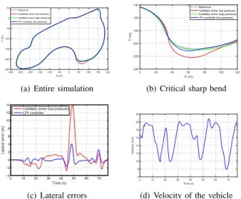
(21b) The path of the vehicle is illustrated in Figure 4(a). It can be seen that the built-in CarMaker driver model is able to follow the track when the tire pressures have nominal values. In most of the simulation the driver model is also able to follow the track with low pressures in the front tires, except for the sharp bend, which is highlighted in Figure 4(b). It means that the tire pressures have significant impact on the maneuverability of the vehicle and the reduction of the pressures can lead to the degradation of the performances.
However, using the designed LPV control, the vehicle can be held on the road track with a significantly reduced lateral error between45−50s, see Figure 4(c). It can be seen that the LPV controller provides smaller error throughout the entire simulation, even if the longitudinal velocity is significantly varied, see Figure 4(d).
-300 -250 -200 -150 -100 -50 0 50 100 150 200 X (m)
-250 -200 -150 -100 -50 0 50
Y (m)
Reference CarMaker driver (low pressure) CarMaker driver (high pressure) LPV controller (low pressure)
(a) Entire simulation
0 20 40 60 80 100 120
X (m) -240
-220 -200 -180 -160 -140
Y (m)
Reference CarMaker driver (low pressure) CarMaker driver (high pressure) LPV controller (low pressure)
(b) Critical sharp bend
0 10 20 30 40 50 60 70
−4
−2 0 2 4 6 8 10 12 14
Time (s)
Lateral error (m)
CarMaker driver (low pressure) LPV controller
(c) Lateral errors
0 10 20 30 40 50 60 70
Time (s) 6
8 10 12 14 16 18 20 22
Velocity (m/s)
(d) Velocity of the vehicle Fig. 4. Positions of the vehicles during the simulations
Figure 5 shows the estimation results of the neural net- work. The illustration shows that the estimation is close to the real pressure 1 bar. However, due to the increased longitudinal and lateral slips in some corners of the track, the estimated pressure may be inaccurate for short time segments. It means that it is necessary to define the vehicle dynamic regions where the results of the estimation are accurate. Experience shows that the estimation is executed if the following criterion is satisfied:
|β|<0.075 radand|ψ|˙ <0.5rad. (22) When the conditions are not satisfied, the last acceptable value is considered in the LPV design. Generally, when the pressures of the tires change slowly, the assumption is acceptable. The blue solid line shows the cases when the conditions are satisfied, while the red dashed line represents the further cases. In the region of the acceptable region the the estimation is accurate, its mean error is below<0.03.
0 10 20 30 40 50 60 70
0 0.5 1 1.5
Front left tire pressure (bar)
0 10 20 30 40 50 60 70
Time (s) 0
0.5 1 1.5 2
Front right tire pressure (bar)
Fig. 5. Result of the pressure estimation
Using the actual value of the tire pressure and the ve- locity information, the LPV control computes the steering angle and the differential torque. The steering angles of the CarMaker Driver and the LPV control scenarios are shown in Figure 6(a). It can been seen that the LPV system provides slightly lower values than the CarMaker Driver, with which the stable motion of the vehicle is reached. Furthermore, the
impacts of the lower steering values are increased with the torque of the differential drive on the rear axle, as it is shown in Figure 6(b).
0 10 20 30 40 50 60 70 80
Time (s) -0.4
-0.3 -0.2 -0.1 0 0.1 0.2 0.3 0.4 0.5 0.6
Steering angle (rad)
CarMaker driver LPV controller
(a) Steering intervention
0 10 20 30 40 50 60 70
Time (s) -1000
-500 0 500 1000 1500
CoG torque (Nm)
(b) Differential drive actuation Fig. 6. Control inputs of the system
V. CONCLUSIONS
The paper has proposed a novel integration of tire pres- sure estimation and path-following control design based on machine learning and LPV methods. The effectiveness of the tire pressure estimator has been examined at various types of measured signals. It has been concluded that the neural network can be effective at the consideration of the measured signals with their past values. Moreover, an LPV based control design method has been introduced, in which the impact of the tire pressure through a scheduling variable has been considered. The results of the comprehensive sim- ulation studies have demonstrated that the integration of the estimator and the LPV controller has been able to handle the critical situations at varied tire pressures.
REFERENCES
[1] S. Velupillai and L. Guvenc, “Tire pressure monitoring [applications of control],”IEEE Control Systems Magazine, vol. 27, no. 6, pp. 22–25, Dec 2007.
[2] C. R. Bowen and M. H. Arafa, “Energy harvesting technologies for tire pressure monitoring systems,”Advanced Energy Materials, vol. 5, no. 7, p. 1401787, 2015.
[3] J. Qian, D.-S. Kim, and D.-W. Lee, “On-vehicle triboelectric nano- generator enabled self-powered sensor for tire pressure monitoring,”
Nano Energy, vol. 49, pp. 126 – 136, 2018.
[4] S. Solmaz, “A novel method for indirect estimation of tire pressure,”
9th Asian Control Conference (ASCC), 2013.
[5] J. Siegel, R. Bhattacharyya, S. Sarma, and A. Deshpande,
“Smartphone-based vehicular tire pressure and condition monitoring,”
inProceedings of SAI Intelligent Systems Conference (IntelliSys) 2016.
IntelliSys 2016. Lecture Notes in Networks and Systems, vol. 15, 2015, pp. 446–455.
[6] F. Wang, H. Chen, H. Guo, and D. Cao, “Constrained h8 control for road vehicles after a tire blow-out,”Mechatronics, pp. 371–382, 2015.
[7] H. Guo, F. Wang, H. Chen, and D. Guo, “Stability control of vehicle with tire blowout using differential flatness based mpc method,”
Proceedings of the 10th World Congress on Intelligent Control and Automation, pp. 2066–2071, 2012.
[8] H. B. Pacejka, Tyre and vehicle dynamics. Oxford: Elsevier Butterworth-Heinemann, 2004.
[9] M. Nielsen,Neural Networks and Deep Learning. Determination Press, 2015.
[10] S. Arlot and A. Celisse, “A survey of cross-validation procedures for model selection,”Statist. Surv., vol. 4, pp. 40–79, 2010.
[11] M. Hagan, H. Demuth, and M. Beale, Neural Network Design.
Boston: PWS Publishing, 1996.
[12] P. G´asp´ar, Z. Szab´o, J. Bokor, and B. N´emeth,Robust Control Design for Active Driver Assistance Systems. A Linear-Parameter-Varying Approach. Springer Verlag, 2017.
[13] R. Rajamani, “Vehicle dynamics and control,”Springer, 2005.
[14] L. Ljung,System identification: theory for the user. USA: Prentice- Hall, 2003.