LPV-based autonomous vehicle control using the results of big data analysis on lateral dynamics
D´aniel F´enyes, Bal´azs N´emeth, P´eter G´asp´ar
Abstract— The paper presents a new big data based control design for autonomous vehicles. The main contribution of this work is the longitudinal velocity optimization process, which is based on the approximation of the reachability sets of a passenger vehicle by using a machine-learning approach.
The data, which is used for the approximation, is provided by the high-fidelity car simulation software, CarSim. The approximation is performed by applying a well-known decision tree algorithm, C4.5. The reachability sets are computed for different longitudinal velocities. Moreover, a LPV technique based lateral control design is proposed, which is used to guarantee the trajectory tracking of the vehicle. To enhance the capability of the LPV controller, the control scheme is extended with the longitudinal velocity optimization process. Thus, the stable and safe motion of the vehicle is guaranteed.
I. INTRODUCTION AND MOTIVATION
The development of the autonomous vehicles has brought new challenges for the whole automotive industry and the control engineers. The automated vehicles requires more accurate sensors, decision making algorithms and advanced control solutions. Since the dynamics of the vehicle is highly nonlinear and cannot be modeled accurately due to the uncertainties, the conventional control methods cannot provide robust and reliable solutions for this problem. In the recent years, the new artificial intelligence (AI) based and other traditional machine learning (or big data) methods have become popular among control engineers. They can be used for a variety of problems including: state estimation, object recognition and even for control problems, such as tracking of a predefined signal, see e.g., [1], [2], [3]. Most of the machine learning and artificial intelligence methods require a lot of data for teaching their models. Fortunately, the modern vehicles are getting equipped with more and more sensors, which measure a lot of information about the car. From the measurements of the individual vehicles, gigantic databases
B. N´emeth, P. G´asp´ar and D. F´enyes are with Systems and Con- trol Laboratory, Institute for Computer Science and Control, Hungarian Academy of Sciences, Kende u. 13-17, H-1111 Budapest, Hungary.E-mail:
[daniel.fenyes;balazs.nemeth;peter.gaspar]@sztaki.mta.hu
The work was supported by the research program titled ”Exploring the Mathematical Foundations of Artificial Intelligence (2018-1.2.1-NKP- 00008).
The research was supported by the Hungarian Government and co- financed by the European Social Fund through the project ”Talent manage- ment in autonomous vehicle control technologies” (EFOP-3.6.3-VEKOP- 16-2017-00001).
The work of B. N´emeth was partially supported by the J´anos Bolyai Re- search Scholarship of the Hungarian Academy of Sciences and the UNKP- 19-4 New National Excellence Program of the Ministry for Innovation and Technology. The work of D. F´enyes was partially supported by the UNKP- 19-3 New National Excellence Program of the Ministry for Innovation and Technology.
can be created. These databases can provide good bases for machine learning algorithms and big data analyses, see [4].
Several papers utilize these huge amount of information.
For example in [5], a pace regression based solution can found for the estimation of the side-slip angle of the vehicle.
Another example is given in [6], which describes a machine learning algorithm based method for the determination of the road surface. The machine learning methods can also be used for computing the reachability sets of the vehicle, see [7]. Furthermore, [8] presents an MPC (Model Predic- tive Control) scheme, which is extended with the result of the big data analysis. This paper presents a method to determine the reachability sets of the vehicle, which are used in the computation of the optimal longitudinal velocity profile. Furthermore, a Linear Parameter Varying (LPV) based lateral control design is proposed for autonomous vehicles. The control structure is extended with a velocity profile optimization process, which can guarantee the safe and stable motion of the vehicle. The velocity optimization process utilizes the reachability sets of the vehicle, which are determined by using a machine learning method, more precisely the decision tree algorithm, called C4.5. The paper describes the acquisition of the data, which is the basis of the determination of the reachability sets. Furthermore, the prepocess steps of the acquired data are also presented. The main contributions of the paper are the LPV-based lateral control design and the longitudinal velocity optimization algorithm.
autonomous vehicle
big data
collection preprocess reachability set approximation
LPV steering control
velocity profile optimization
Longitudinal controller
vx,ref
Longitudinal actuation Steering actuation
Reachabilitysets
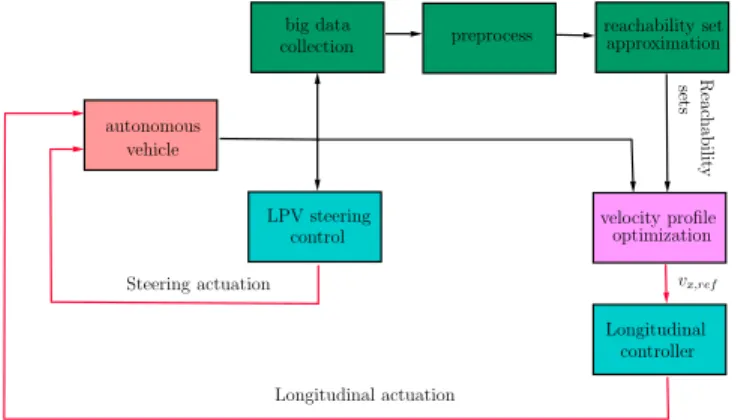
Fig. 1. Scheme of the proposed control structure
The structure of the proposed autonomous vehicle control solution is illustrated in Figure 1. As a first step, the collection of the dataset must be done. Then, the collected raw data has to be prepared for the further data analysis steps.
2020 American Control Conference Denver, CO, USA, July 1-3, 2020
The prepared dataset is used for computing the reachability sets of the vehicle, which will serve as the basis of the velocity optimization algorithm. The block ’LPV steering control’ represents the design of a lateral tracking control algorithm, which is based on the LPV framework. Whilst, the ’Longitudinal controller’ is responsible for guaranteeing the realization of the computed optimal velocity profile. The longitudinal controller is based on a simple PID structure, therefore it’s not detailed in this paper.
The remainder of the paper is structured as follows.
Section II presents the data acquisition, the preprocess of the data and the computation of the reachability sets. The next section details the LPV-based lateral control design and the longitudinal velocity optimization process. Finally, the last section shows a comprehensive simulation to show the operation and effectiveness of the proposed control scheme.
II. BIG DATA ANALYSIS ON LATERAL DYNAMICS
In this section, the determination of the reachability sets of the vehicle is presented by using a machine learning approach. For the computation of the reachability sets a well- known decision tree algorithm is applied, which is called C4.5. Furthermore, the acquisition of the datasets and the prepocess of the raw data are also detailed in this section.
Acquisition of dataset
The first step of any data-based analysis is the acquisition of the appropriate dataset. In this research, the dataset is provided by the high fidelity simulation software, CarSim.
In the simulations the test vehicle has been controlled by the CarSim’s built-in driver model. Several simulations have been conducted using different parameter sets. During the simulations the following parameters have been changed:
longitudinal velocity, adhesion coefficient, simulation track.
From the simulations, only those variables/measurements have been save, which could be measured in all modern cars, such as:
• Longitudinal velocity (vx)
• Yaw-rate (ψ)˙
• Accelerations (ax, ay)
• Wheel speeds (ωf l, ωf r, ωrl, ωrr)
• Side-slip angle (β) (for illustration purposes)
• Adhesion coefficientµ (Simulation parameter)
In this manner, more than 10 million instances have been collected and saved.
Prepocessing of dataset
The measurements and other information, which are pro- vided by car’s sensors, require some preprocess steps before using them in any machine learning algorithms. These steps, for example, includes the selection of the relevant signals (variable). Since not all of the measured attributes must be used (or necessary) for a given machine learning based problem, the selection of the most significant ones is a crucial step. Another problem is the selection of the stable instances.
Since the reachability sets contain only the stable states of a given system, an appropriate criterion must be found to
split the measured instances into stable and unstable groups.
In the literature, several criteria can be found that can give information on the stability of the vehicle e.g. [9], [10].
Unfortunately, they do not fit for this classification problem.
Therefore, a new criterion is used, which is based on the linearized one-track lateral model, see [11], [12], [13].
The basic idea behind this criterion is that the motion of the vehicle is considered to be stable, when its dynamical behavior is close to the linear region. Thus, the criterion is formed as the deviation of the actual vehicle motion and the linear model, which can be expressed as:
−ε1< |1 +α1|
|1 +δ−β−lv1ψ˙
x|
−1≤ε1, (1) whereα1 is the averaged side-slip angle of the front wheels, δis the averaged steering angle of the front wheels,βdenotes the side-slip angle of the CoG of the vehicle,ψ˙represents the yaw-rate of the vehicle,l1 is the distance between the front axis and the CoG and vx is the longitudinal velocity of the vehicle. Moreover,ε1is an experimentally defined parameter.
An instance is considered to be stable, if it satisfies the inequality (1), while in the other case, it said to be unstable.
Approximation of the reachability sets
As mentioned earlier, the so-called C4.5. decision tree algorithm is used to determine the reachability sets of the vehicle. In this subsection a brief introduction is given to this method, see [14], [15]. The result of the algorithm is a decision tree, which can determine that whether an instance belongs to the group, which contains the stable instances, or not. A decision tree has three main components:
1) Nodes: They represents a condition e.g.: the value of an variable is bigger or smaller than a given value. The outcome of a node can lead to another node or to a leaf.
2) Branches:The nodes and the leaves are connected by branches. A branch connects the outcome of a node to another node or to a leaf.
3) Leaves: Finally, the leaves determine the class of the instances. In this case, the leaves separate the instances into stable and unstable groups.
The C4.5 algorithm was developed by R. Quinlan in 1993, detailed descriptions can be found in [15] and [16]. The de- cision tree algorithm C4.5 uses the metric called information gain to optimize the generated decision tree. Furthermore, a crucial parameter of the algorithm is the ’number of minimal objects per leaf’. This parameter influences the size of the generated tree. If the value of this parameter is set to a small number, in general, the resulted tree consists of a huge number of nodes and leaves. In the other case, the number of the components can be reduced by setting this parameter to a small value. Therefore, the size of the decision tree can be controlled by this parameter, which is especially useful when the decision trees are used in any control system.
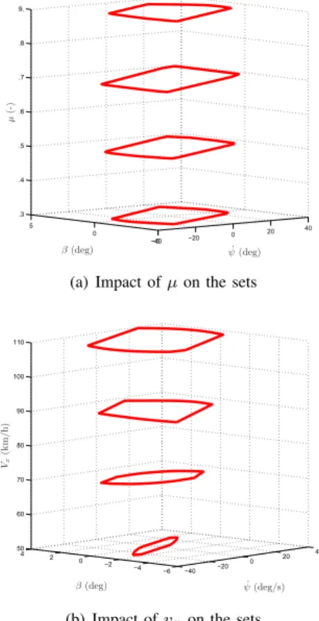
The results of the decision tree are illustrated in Figures 2. Only the instances, which are classified as stable by the
decision tree, are depicted. Moreover, in the figures the stable instances are approximated by a convex hull, which is a conservative inner approximation of the reachability sets. As the figures shows the reachability sets, which are illustrated in the plane of ψ˙ (yaw-rate) and β (side-slip angle) with respect to the adhesion coefficient (µ) in the top figure and to the longitudinal velocity (vx) in the second figure. It can be observed that the shapes and the sizes of the reachability sets can change along with the velocity and the adhesion coefficient. This means that the intervention of the vehicle must be fitted to the actual circumstances.
−40 −20 0 20 40
−5 0 5 .3 .4 .5 .6 .7 .8 9.
µ(-)
ψ˙(deg) β(deg)
(a) Impact ofµon the sets
−40 −20 0 20 40
−4 −6 0 −2 4 2 50 60 70 80 90 100 110
Vx(km/h)
β(deg) ψ˙(deg/s)
(b) Impact ofvxon the sets
Fig. 2. Illustration of the reachability set approximations
III. LPV-BASED VEHICLE CONTROL DESIGN AND VELOCITY SELECTION STRATEGY
This section focuses on the lateral control design and longitudinal velocity optimization for autonomous vehicles.
The main goal of these algorithms is to create an enhanced control scheme, which is able to guarantee the safe and stable motion of the vehicle. The lateral control design is based on the LPV (Lateral Parameter Varying) approach, in which the longitudinal velocity is used as a scheduling parameter.
Whilst, in the velocity optimization process, the presented reachability sets are utilized to compute the optimal velocity profile.
Design of lateral LPV control
In the lateral control design, the one-track lateral vehicle model is used, whose detailed description can be found in
[11]. The model consists of the following three equations:
mvx( ˙ψ+ ˙β) =Fy(α1) +Fy(α2), (2) Jψ¨=Fy(α1)l1−Fy(α2)l2, (3)
˙
vy=vx( ˙ψ+ ˙β), (4) where β denotes the side-slip angle of the vehicle, ψ˙ represents the yaw-rate of the vehicle, vx and vy are the longitudinal and lateral velocities of the vehicle, l1, l2 are the distances between the axes and CoG of the vehicle, whilemis the mass of the vehicle andJ is the yaw inertia.
Furthermore, Fy denotes the lateral force of the tires, see [17]. They depend the side slips of the tires (α1, α2). In this case, this relationship is considered to be linear, therefore it can be approximated as Fy = Cαi. C is the cornering stiffness.
Using these equations, the following state-space represen- tation can be derived:
˙
x=A(ρ1)x+B(ρ1)u, (5) whose state-vector consists of x = ψ˙ β vy yT
, the actuation isu=δ and ρ1 =vx is the scheduling variable.
Moreover, A(ρ1), B(ρ1) are matrices of system (5). The lateral control design has two main goals: 1./ To ensure the safe and the stable trajectory tracking of the vehicle, 2./ To minimize the actuation of the system. These goals form the following performances:
• Minimization of the lateral error:
One of the main goals of the controller is to guarantee the trajectory tracking of the vehicle, which means that the controller must minimize the error between the actual lateral position (y) and reference signal (yref):
z1=yref −y, |z1| →min. (6)
• Minimization of the actuation:
The mentioned trajectory tracking must be reached by using minimal energy (intervention):
z2=δ, |z2| →min. (7) These performances are summed up by the performance vec- tor:z=
z1 z2T
, which forms the performance equation:
z=C1x+D11r+D12u, (8) whereC1, D11, D12are matrices andrcontains the reference signalyref.
The LPV-based control design aims to find a controller that can ensure the balance between the presented performances and the external noises. The optimal balance between the performances can be reached by using scaling or weight- ing functions. The structure of the closed-loop system is illustrated in Figure 3. As it can be seen, several weighting functions are used to guarantee the predefined performances of the system. The goal ofWref,1is to weight the reference signal in such a manner to ensure the smooth tracking.
Wz1 represents the weight of the first performance, which means it is responsible for the tracking of the lateral position.
The weighting functionWz2 is to minimize the intervention (steering angle) of the system. Finally,Wω,1 attenuates the external noise on the measured signal.
P(ρ1)
K(ρ1)
measuredvehiclesignals
ρ1 velocity selection
Wref,1 yref
y
δ
Wz,1
Wz,2
z1
z2
Ww,1 wy
Fig. 3. Closed-loop interconnection structure
The quadratic LPV performance problem is to choose the parameter-varying controller K(ρ1) in such a way that the resulting closed-loop system is quadratically stable and the inducedL2norm from the disturbance and the performances is less than the value γ. The minimization task is the following:
K(ρinf1) sup
ρ1,∈Fρ
sup
kwk26=0,w∈L2
kzk2
kwk2, (9) whereFρbounds the scheduling variables. The optimization problem is solved by using the LPVTools in MATLAB environment, see [18]. The yielded controller K(ρ1) is formed as
˙
xK =AK(ρ1)xK+BK(ρ1)yK, (10) u=CK(ρ1)xK+DK(ρ1)yK, (11) where xK is the state vector of the dynamic controller, AK, BK, CK, DK are ρ1 dependent matrices. yK is the vector of the lateral error and yaw-rate error measurements, which is formed as
yK=C2x+D21r, (12) whereC2, D21 are matrices.
The existence of a controller that solves the quadratic LPV γ-performance problem can be expressed as the feasibility of a set of LMIs, which can be solved numerically. The constraints set by the LMIs are not finite. The infiniteness of the constraints is relieved by a finite, sufficiently fine grid.
To specify the grid of the performance weights for the LPV design the scheduling variables are defined through lookup- tables, see [19], [20].
Design of the optimal velocity profile
The goal of the velocity profile optimization is to guaran- tee the safe and stable motion of the vehicle. It means that the state of the vehicle remain close to the linear region of its dynamics. This condition can be ensured by keeping the states of the vehicle inside the reachability sets. Of course,
the ultimate goal is to maximize the longitudinal velocity, while keeping the states inside the reachability sets.
For guaranteeing this criterion, the prediction of the mo- tion of the vehicle, especially the states ψ˙ (yaw rate) and β (side-slip angle) must be computed. This can be made by forming the closed-loop system using the nominal LPV model (2) and the controller (10).
˙
xcl=Acl(ρ1)xcl+Bcl(ρ1)r, (13) wherex˙cl=
˙ x x˙KT
and the components are Acl(ρ1) =
Acl,11 Acl,12
Acl,21 Acl,22
, (14)
Bcl(ρ1) =
B(ρ1)DK(ρ1)D21
BK(ρ1)D21
. (15)
with the following matrices
Acl,11=A(ρ1) +B(ρ1)DK(ρ1)C2, Acl,12=B(ρ1)CK(ρ1),
Acl,21=BK(ρ1)C2, Acl,22=AK(ρ1),
In order to predict the motion of the vehicle, the presented closed-loop system must be discretized using the sample time T, detailed explanation can be found in [21]:
xcl(k+ 1) =Acl(k)xcl(k) +Bcl(k)r(k), (16) ycl(k) =Cclxcl(k), (17) where Acl(k), Bcl(k) are used as compact notations of Acl(ρ1(k))andBcl(ρ1(k)). Moreover,ycl(k)containsψ˙and β, and Ccl is the corresponding matrix. The prediction of ycl(k)can be computed on a n-steps long horizon as:
ycl(k, n)=
ycl(k+ 1) ycl(k+ 2)
... ycl(k+n)
=A+BR, (18)
where
A=
CclAcl(k) CclAcl(k)Acl(k+ 1)
... Ccl
k+n
Q
i=k
Acl(i)
xcl(k) (19)
B=
CclBcl(k) · · · 0 CclAcl(k)Bcl(k) · · · 0
... . .. ...
Ccl k+n−1
Q
i=k
Acl(i)Bcl(k) · · · CclBcl(k)
(20)
R=
r(k+ 1) ... r(k+n)
. (21)
-200 -100 0 100 200 300 400 X coordinate (m)
-200 -150 -100 -50 0 50 100 150
Y coordiante (m)
Fig. 4. Michigan track
Using these notations, the optimization problem can be formed. The main goal of the velocity profile de- sign is to maximize the elements of the vector ρ = ρ1(k+ 1). . . ρ1(k+n)T
, which contains the reference longitudinal velocity on the forthcoming road segments. Of course, the elements of this vector have upper bounds, which can be handled as constraints during the optimization process
ρ≤ρmax. (22)
ρmaxcontains the upper bounds of the longitudinal velocity on the forthcoming road horizon. The stability of the vehicle can be guaranteed by ensuring that the predicted states of the vehicle ycl(k, n) remain inside the reachability sets, presented in Section II. This criterion can be formed as:
ycl(k, n)∈ R ρ1(i)
, ∀k≤i≤n. (23) Then, the final optimization task is:
ρ1(k+1)...ρmax1(k+n)ρ (24) subject to the constraints (22), (23):
ρ≤ρmax (25)
ycl(k, n)∈ R ρ1(i)
, ∀k≤i≤n. (26) The solution of the optimization is a vector, which contains the optimized velocity profile for nsteps ahead.
IV. SIMULATION EXAMPLES
In this section a comprehensive simulation examples is presented to show the operation and the effectiveness of the proposed control algorithm. The analysis has been performed using the Weka data mining software [22], while the dataset has been collected through the CarSim vehicle dynamic simulator.
The vehicle, which is used in the simulation, a D-class passenger car, whose mass is m = 2015kg. During the simulation, the vehicle is driven along a segment of Michigan Waterford Hills Road Racing track twice, see IV. In the first run, the vehicle uses the optimized velocity profile, while in the second simulation, the car uses the nominal velocity profile.
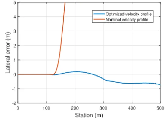
The results of the simulations are illustrated in the follow- ing figures. Figure 5 shows the lateral error for both cases. As it can be seen the vehicle, which uses the original velocity profile, leaves the road at 120m. At that station, a sharp bend begins, which cannot be tracked by the vehicle with the predefined velocity profile. In the first case, the car is able to track the road at the sharp bend since the original velocity profile is overwritten by the velocity optimization process.
0 100 200 300 400 500
Station (m) -2
-1 0 1 2 3 4 5
Lateral error (m)
Optimized velocity profile Nominal velocity profile
Fig. 5. Lateral error of the vehicles on Waterford Hills track
The modified velocity profile is illustrated in Figure 6.
It can be seen that the algorithm reduces the longitudinal velocity after 6s, which reflects on the mentioned sharp bend.
0 5 10 15 20 25 30 35
Time (s) 0
5 10 15 20 25
vx (m/s)
Fig. 6. Velocity profiles
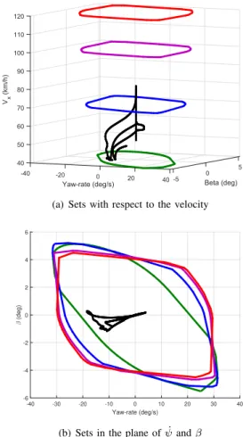
The Figures 7 show the states of the vehicle in the plane of ψ˙ (yaw-rate) andβ (side-slip angle) for that case when the modified velocity profile is used. As the figures indicate, the states of the vehicle do not leave the stable region of its states, therefore the stability of the vehicle is guaranteed throughout the simulation. Furthermore, this is the reason why the vehicle does not leave the road in the first case.
Finally, the Figure 8 shows the steering actuation in the simulation. The steering angle is between[−4,1deg], which is a reasonable range for this system.
V. CONCLUSIONS
The paper has presented a LPV bases lateral control design for autonomous vehicles. The control system has been
40 5
0 50
-40
Beta (deg) 60
70 80 90
Vx (km/h) 100 110 120
-20 0
Yaw-rate (deg/s) 20 40-5
(a) Sets with respect to the velocity
-40 -30 -20 -10 0 10 20 30 40
Yaw-rate (deg/s) -6
-4 -2 0 2 4 6
(deg)
(b) Sets in the plane ofψ˙andβ
Fig. 7. Reachabaility sets and the trajectory of the vehicle
extended with a longitudinal velocity profile optimization process. This algorithm utilized the reachability sets of the vehicle, which had been determined by using a decision tree algorithm, called C4.5. Furthermore, a comprehensive simulation example has been presented to show the operation and the effectiveness of the proposed control algorithm. In the simulations, two cases have been compared to each other.
In the first case, the vehicle has used the original velocity profile, while in the second case the car has been driven by the modified profile. It has been shown that without the modified velocity the vehicle was not able to follow the predefined path.
REFERENCES
[1] J. Jeon, W. Lee, H. J. Cho, and H. Lee, “A big data system design to predict the vehicle slip,” in15th Int. Conf. Control, Automation and Systems (ICCAS), 2015.
[2] H. A. Najada and I. Mahgoub, “Autonomous vehicles safe-optimal trajectory selection based on big data analysis and predefined user preferences,” in7th Annual Ubiquitous Computing, Electronics Mobile Communication Conference, 2016.
[3] M. Zhu, X. Y. Liu, M. Qiu, R. Shen, W. Shu, and M. Y. Wu, “Traffic big data based path planning strategy in public vehicle systems,” in 24th Int. Symp. Quality of Service, 2016.
[4] W. Xu, H. Zhou, N. Cheng, F. Lyu, W. Shi, J. Chen, and X. Shen,
“Internet of vehicles in big data era,”IEEE/CAA Journal of Automatica Sinica, vol. 5, no. 1, pp. 19–35, Jan 2018.
0 5 10 15 20 25 30 35
Time (s) -4
-3 -2 -1 0 1
(deg)
Fig. 8. Steering angle actuation
[5] D. F´enyes, B. N´emeth, M. Asszonyi, and P. G´asp´ar, “Side-slip angle estimation of autonomous road vehicles based on big data analysis,”
in26th Mediterranean Conference on Control and Automation, 2018.
[6] D. Fenyes, B. Nemeth, P. Gaspar, and Z. Szabo, “Road surface estimation based lpv control design for autonomous vehicles,”Proc.
3rd IFAC Workshop on Linear Parameter Varying Systems, Eindhoven, Netherlands.
[7] D. Fenyes, B. Nemeth, and P. Gaspar, “A predictive control for au- tonomous vehicles using big data analysis,”Proc. 9th IFAC Symposium on Advances in Automotive Control, Orleans, France, 2019,.
[8] ——, “Impact of big data on the design of mpc control for autonomous vehicles,” Proc. 18th European Control Conference Napoli, Italy, 2019.
[9] S. Sadri and C. Wu, “Stability analysis of a nonlinear vehicle model in plane motion using the concept of lyapunov exponents,”Vehicle System Dynamics, vol. 51, no. 6, pp. 906–924, 2013.
[10] B. N´emeth, P. G´asp´ar, and T. P´eni, “Nonlinear analysis of vehicle control actuations based on controlled invariant sets,”Int. J. Applied Mathematics and Computer Science, vol. 26, no. 1, 2016.
[11] R. Rajamani, “Vehicle dynamics and control,”Springer, 2005.
[12] D. F´enyes, B. N´emeth, and P. G´asp´ar, “Analysis of autonomous vehicle dynamics based on the big data approach,” in European Control Conference, 2018.
[13] M. Masouleh and D. Limebeer, “Region of attraction analysis for non- linear vehicle lateral dynamics using sum-of-squares programming,”
Vehicle System Dynamics, vol. 56, no. 7, 2018.
[14] E. B. Hunt,Concept Learning: An information Processing Problem.
Wiley, 1962.
[15] J. R. Quinlan,C4.5: Programs for Machine Learning. San Mateo, California: Morgan Kaufmann Publishers, 1993.
[16] ——, “Bagging, Boosting, and C4.5,”Proceedings of the Thriteenth National Conference on Artificial Intelligence, pp. 725–730, 1996.
[17] R. Ghandour, A. Victorino, M. Doumiati, and A. Charara, “Tire/road friction coefficient estimation applied to road safety,”18th Mediter- ranean Conference on Control and Automation, 2010.
[18] G. Balas, A. Hjartarson, A. Packard, and P. Seiler, “A toolbox for modeling, analysis, and synthesis of parameter varying control systems,” 2015.
[19] F. Wu, X. Yang, A. Packard, and G. Becker, “Induced L2 norm controller for LPV systems with bounded parameter variation rates,”
Journal of Robust and Nonlinear Control, vol. 6, pp. 983–988, 1996.
[20] Z. Szab´o, A. Marcos, D. P. Mostaza, M. Kerr, G. R¨od¨onyi, J. Bokor, and S. Bennani, “Development of an integrated LPV/LFT framework:
modeling and data-based validation tool,” IEEE Transactions on Control Systems Technology, vol. 19, no. 1, pp. 104–117, 2011.
[21] R. T´oth, Modeling and Identification of Linear Parameter-Varying Systems, ser. Lecture Notes in Control and Information Sciences.
Berlin, Heidelberg: Springer, 2010, vol. 403.
[22] I. Witten and E. Frank,Data Mining Practical Machine Learning Tools and Techniques. Morgan Kaufmann Publishers, Elsevier, 2005.