Brain Tumor Segmentation from Multi-Spectral MRI Data Using Cascaded Ensemble Learning*
T´ımea F¨ul¨op, ´Agnes Gy˝orfi, Szabolcs Csaholczi, Levente Kov´acs and L´aszl´o Szil´agyi
Abstract— Ensemble learning methods are frequently em- ployed in medical decision support. In image segmenta- tion problems the ensemble based decisions require a post- processing, because the ensemble cannot adequately handle the strong correlation of neighbor voxels. This paper proposes a brain tumor segmentation procedure based on an ensemble cascade. The first ensemble consisting of binary decision trees is trained to separate focal lesions from normal tissues based on four observed and 100 computed features. Starting from the intermediary labels provided by the first ensemble, six local features are computed for each voxel that serve as input for the second ensemble. The second ensemble is a classical random forest that enforces the correlation between neighbor pixels, regularizes the shape of the lesions. The segmentation accuracy is characterized by 85.5% overall Dice Score, 0.5%
above previous solutions.
Index Terms— Image segmentation, brain tumor segmenta- tion, magnetic resonance imaging, ensemble learning.
I. INTRODUCTION
The number of active medical imaging devices is steadily growing. The amount of medical image data created by these devices is rising even quicker. On the other hand, the number of human experts who can evaluate the medical image data cannot follow this growing trend. Consequently, there is a strong need for automatic image segmentation and interpretation algorithms that can reliably process the large mass of medical records and select those suspected ones, which should be inspected by the human experts.
Multi-spectral magnetic resonance imaging (MRI) is the medical imaging modality usually employed in brain tumor
*This project was supported in part by the Sapientia Institute for Research Programs. This project has received funding from the European Research Council (ERC) under the European Unions Horizon 2020 research and innovation programme (grant agreement No 679681). The work of T. F¨ul¨op was supported by the Collegium Talentum 2019 Programme of Hungary. The work of L. Szil´agyi was supported by the Hungarian Academy of Sciences through the J´anos Bolyai Fellowship program.
T. F¨ul¨op and Sz. Csaholczi are with Dept. of Mathematics- Informatics, Sapientia University, Calea Sighis¸oarei 1/C, 540485 Tˆırgu Mures¸, Romania (phone: +40-265-206-210; fax: +40-265-206-211; e- mail: {fuloptimea1427,szabolcscsaholczi55} at gmail.com).
A. Gy˝orfi is with Doctoral School of Applied Informatics, ´´ Obuda Univer- sity, B´ecsi ´ut 96/b, H-1034 Budapest, Hungary (phone/fax: +36-1-666-5585;
e-mail:gyorfi.agnes at phd.uni-obuda.hu).
L. Kov´acs and L. Szil´agyi are with University Research, Innovation, and Service Center (EKIK), ´Obuda University, B´ecsi ´ut 96/b, H-1034 Budapest, Hungary (phone/fax: +36-1-666-5585; e-mail: {kovacs.levente, szilagyi.laszlo} at nik.uni-obuda.hu).
A. Gy˝orfi and L. Szil´agyi are also with Dept. of Electrical En-´ gineering, Sapientia University, Calea Sighis¸oarei 1/C, 540485 Tˆırgu Mures¸, Romania (phone: +40-265-206-210; fax: +40-265-206-211; e-mail:
{gyorfiagnes,lalo} at ms.sapientia.ro).
detection and segmentation [1]. The development of auto- matic detection and segmentation algorithms for the brain tumor has been intensively investigated, as a consequence of the BraTS Challenges organized yearly since 2012 [2], [3]. The whole methodology arsenal of pattern recognition is involved in this process. Most solutions employed machine learning techniques, supervised and semi-supervised ones, sometimes combined with advanced image segmentation tools, like: ensemble of random forests [4], AdaBoost clas- sifier [5], random forests [6], [7], [8], extremely random trees [9], support vector machines [10], convolutional neural network [11], [12], deep neural networks [13], [14], [15], Gaussian mixture models [16], fuzzy c-means clustering in semi-supervised context [17], [18], tumor growth model [19], and various advanced image segmentation techniques like cellular automata combined with level sets [20], active contour models [21] combined with texture features [22], and graph cut algorithm [23]. The review paper published by Gordilloet al.in [24] is a fine summary of the solutions produced in the pre-BraTS era.
This paper proposes a two-step ensemble learning based procedure for the detection and segmentation of brain tu- mors from MRI data. The first ensemble of binary decision trees produces an intermediary labeling of voxels using the observed MRI intensity values and several further computed features. The second ensemble is a classical random forest which produces the final decision starting from six features computed from the local distribution of intermediary labels.
The rest of this paper is structured as follows: section II presents the details of the proposed segmentation procedure, section III describes the experimental validation of the pro- posed method, while section IV concludes the study.
II. MATERIALS AND METHODS
Previously, we introduced a brain tumor segmentation procedure that used ensemble learning by the means of binary decision trees (BDT), and employed a morphological criterion to enhance the accuracy of lesion segmentation [25], [26]. Later we performed several experiments to improve the overall segmentation quality and the runtime efficiency, like finding an optimal subset of features [27], comparing several types of ensembles [28], searching for the histogram uniformization technique that is most suitable to detect focal lesions [29], including multi-atlases in the segmentation process [30], and determining the effect of feature vector’s spectral resolution upon segmentation accuracy [31]. In this paper we propose a new method that involves a second learn- ing ensemble to provide a better performing segmentation
Statistical evaluation
Morphological post−processing
Random forest based post−processing
Prediction by ensemble Preprocessing :
histogram normalization feature extraction
Atlas based feature enhancement
Train data sampling for ensemble learning
Training the selected ensemble
- - -
-
? MRIdata
Dicescores
Fig. 1. The whole segmentation procedure, highlighting the proposed modification.
criterion at post-processing. The whole modified procedure is depicted in Fig. 1.
A. Data
This study used the nV = 54 low-grade tumor volumes of the MICCAI Brats 2015 train data set [2] to train and test the proposed segmentation procedure. Each volume consist of 155 slices, each slice containing240×240voxels. Voxels have four observed features (T1, T2, T1C, and FLAIR) and the ground truth provided by human experts. In case of each record, all data channels were registered to the T1 channel using an automatic algorithm, and any voxels representing irrelevant (non-brain) tissues were removed [2]. Records were randomly separated into two equal groups that were employed as train and test data in turns.
B. The initial segmentation procedure
The base segmentation procedure that we use as reference is visible in Fig. 1, if we neglect the presence of the high- lighted component. MRI records undergo several processing steps, as listed in the following:
1) Preprocessing has a multiple role: (1) it detects the presence of intensity inhomogeneity [32], [17], [33]
and applies compensation whenever it is necessary using the method of Tustison et al. [34]; (2) it pro- duces uniform histograms to make MRI intensities comparable with each other, accomplished by a con- text sensitive linear transform [29]; (3) it generates 100 computed features (minimum, maximum, average and median intensity values in various neighborhoods;
gradients and Gabor wavelet features) for each voxel, to take advantage from the correlation between neigh- bor voxels and to deal with the imperfection of the automatic registration algorithms that were involved in aligning data channels during the creation of the MICCAI BraTS data set.
2) An ensemble built from nT = 125 decision trees is trained to distinguish normal voxels and the voxels of the whole tumor. Trees are trained using sets os N randomly selected voxels from the train volumes, containing 93% negatives and 7% positives. The proce- dure was evaluated with values of parameterNranging between104 (10k) and106 (1000k). Training uses an entropy criterion to provide optimal decisions. Trees
are not limited in depth so each leaf can give a binary decision. When the ensemble of trees is established, it is used to predict the label of all voxels belonging to the test volumes. The ensemble decision is based on the majority voting of its trees, but this is only an intermediary labeling that serves as input for the post- processing.
3) Morphological post-processing produces the final label of each test voxel based on the intermediary labels of its neighbors: first it establishes the number of positive intermediary labels (νp) and the number of valid brain voxels (ν) within a cubic11×11×11neighborhood of the current voxel. The value of ν cannot exceed 113 and cannot be zero either, because the current voxel is always a valid brain voxel. The rate of positive voxels, determined as ρ = νp/ν, is then compared with a previously defined threshold θ = 1/3. Those voxels are finally assigned positive labels which have ρ > θ, regardless to the voxel’s own intermediary labeling. Post-processing gives the detected tumor a regularized shape and in most cases it enhances the accuracy indicator values.
C. Multi-atlas based enhancement
The segmentation procedure presented so far does not take in consideration the position of the voxels within the volume. In a previous paper [30] we created multiple atlases (one for each feature) based on pixels belonging to normal tissues only, right after the preprocessing steps. Atlas use normalized coordinates, have a cubic shape and a discrete resolution of (2S + 1)×(2S + 1)×(2S+ 1), where S is a parameter. All MRI volumes are aligned to the atlas using a rigid registration technique. For any voxel of the atlas, which have normal brain tissue voxels mapped upon, the average intensity value (μ) and the standard deviation (σ) of intensities is extracted. These local μ and σ values are used to update the original feature values, to map them onto a new target interval, before proceeding to the training and testing of the BDT ensemble. Atlases of various spatial resolutions were tested, with parameterSranging from 60 to 120. All atlases were able to improve segmentation accuracy, best performances were achieved at S∈ {90,100}.
D. The proposed random forest based post-processing In this paper we propose an intelligent, random forest based (RF-based) post-processing method to replace the previous morphological one. The main properties of the proposed solution are presented in the following:
1) The random forest is trained to distinguish positive voxels from negative ones based on six feature, which are computed for all voxels as follow. Let us define five cubic neighborhoods of the current voxel, denoted by Nk, where k = 1. . .5, whose size is (2k+ 1)× (2k+ 1)×(2k+ 1). Within the neighborhood Nk of the current voxel, the number of positive intermedi- ate labels is denoted by νk(p), while the number of valid brain voxels is represented by νk. The rate of positive voxels within neighborhood Nk is computed as ρk = νk(p)/νk. Further on, we define feature η as the normalized value of the number of complete neighborhoods of the current voxel, to be established by the formula:
η= 1 5
5
k=1
δ
νk,(2k+ 1)3
, (1)
where
δ(α, β) =
1 ifα=β
0 otherwise . (2) The feature vector of the current voxels is given as:
(ρ1, ρ2, . . . ρ5, η).
2) The random forest was trained with feature vectors of voxels taken from the high-grade tumor volumes of the MICCAI BraTS data set. A number of107train voxels were randomly selected for the training process.
3) Voxels with feature vectors having ρk = 0 for any k = 1. . .5 are considered negatives by default, such voxels are not used in training and are not fed to the random forest for prediction.
4) The random forest consists of 100 trees, while the maximum depth of each tree was set to 8.
5) The RF-based post-processing uses the implementa- tion provided by the Machine Learning package of OpenCV, version 3.4.0.
E. Evaluation
The segmentation accuracy of each MRI record i (i = 1. . . nV) is primarily expressed by the number of true positives (TPi), false positives (FPi), true negatives (TNi), and false negatives (FNi). Our main accuracy indicator is the Dice Score (DSi), which is computed for any record i as:
DSi= 2×TPi
2×TPi+ FPi+ FNi . (3) Further on, for any MRI recordi, sensitivity (or true positive rate, TPR) is defined as:
TPRi= TPi/(TPi+ FNi) , (4) while specificity (or true negative rate, TNR) is extracted as:
TNRi= TNi/(TNi+ FPi) . (5)
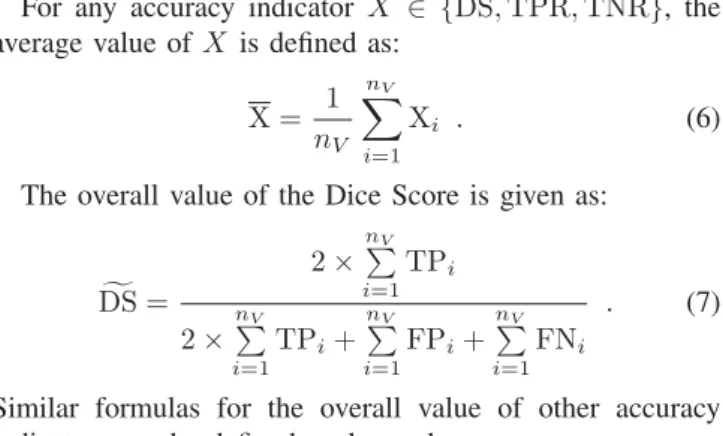
For any accuracy indicator X ∈ {DS,TPR,TNR}, the average value of X is defined as:
X = 1 nV
nV
i=1
Xi . (6)
The overall value of the Dice Score is given as:
DS =
2×nV
i=1TPi 2×nV
i=1TPi+nV
i=1FPi+nV
i=1FNi
. (7)
Similar formulas for the overall value of other accuracy indicators can be defined analogously.
Swapping the role of the train and test data set allows us to have segmentation accuracy indicators for all available low-grade tumor volumes.
III. RESULTS AND DISCUSSION
The above presented brain tumor segmentation procedure, in all its variants, underwent a thorough evaluation involving all 54 low-grade tumor volumes of the BraTS 2015 data set. The train data size varied in four steps, using values of 10k, 100k, 500k, and 1000k. Procedure variants using no atlas and involving atlases of various spatial resolutions (S∈ {60,80,100,120}) were evaluated. The morphological and the RF-based post-processing were evaluated in parallel so that we can formulate comparative assertions. The quality indicators exhibited in Section II-E were extracted for each scenario and each individual MRI record. The average and overall value for each indicator was established for global quality characterization. Results are presented in the follow- ing paragraphs.
Table I presents the main overall accuracy indicator val- ues obtained in case of various train data sizes and atlas resolutions. In each scenario and for each indicator, three values are given: the one obtained without post-processing, the one given by the morphological post-processing, and the one produced by the proposed RF-based post-processing.
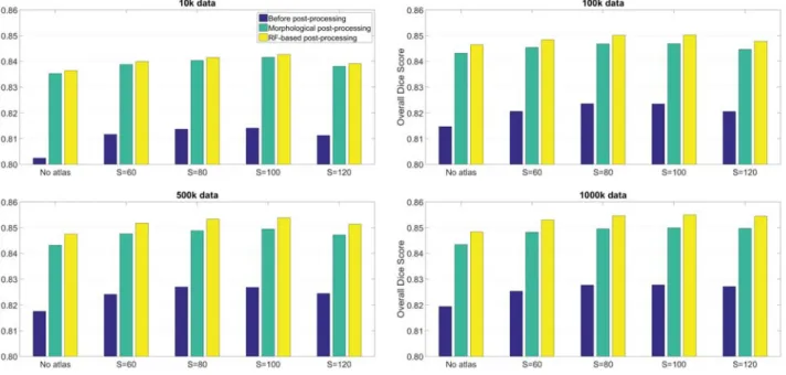
Dice Score, which is the most important accuracy indicator, shows the superiority of the random forest in all cases. The differences rise together with the train data size, from0.1%
at 10k feature vectors per BDT to 0.5%at 1000k data. The best performing atlas is the one represented by S= 100.
Figure 2 exhibits the overall Dice Scores obtained in case of various train data sizes and atlas resolutions, and gives a visual comparison for the values obtained with RF-based and morphological post-processing. Although the difference of only 0.5% may seem small at first sight, that improvement represents the elimination of 9-10% of mistaken labels produced by the morphological post-processing.
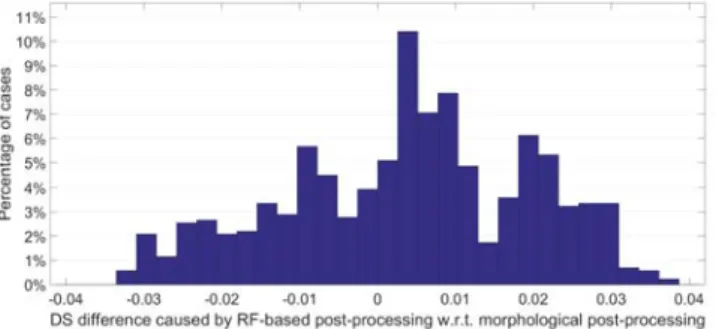
The comparison of Dice Scores obtained for individual MRI records is given in Fig. 3 and Table II. The difference of Dice Scores, the one obtained via RF-based post-processing minus the result of the morphological method, was extracted for all MRI volumes and all scenarios (train data sizes and atlas resolutions). The histogram of all these differences is presented in Fig. 3. The histogram indicated that the
TABLE I
MAIN OVERALL ACCURACY INDICATORS WITHOUT POST-PROCESSING,WITH MORPHOLOGICAL POST-PROCESSING,AND WITH RANDOM FOREST BASED POST-PROCESSING
Train data Atlas Dice Score Sensitivity Specificity
size size BEFORE MORPH RF-BASED BEFORE MORPH RF-BASED BEFORE MORPH RF-BASED
No atlas 0.8024 0.8353 0.8364 0.7277 0.8311 0.8096 0.9934 0.9879 0.9903
S= 60 0.8116 0.8388 0.8399 0.7382 0.8157 0.7943 0.9938 0.9901 0.9926
10k S= 80 0.8137 0.8403 0.8414 0.7383 0.8158 0.7942 0.9942 0.9904 0.9928
S= 100 0.8141 0.8415 0.8426 0.7387 0.8166 0.7951 0.9942 0.9905 0.9929 S= 120 0.8112 0.8380 0.8391 0.7369 0.8143 0.7928 0.9939 0.9901 0.9926
No atlas 0.8147 0.8432 0.8464 0.7466 0.8481 0.8278 0.9934 0.9875 0.9902
S= 60 0.8207 0.8454 0.8484 0.7542 0.8308 0.8104 0.9936 0.9897 0.9924
100k S= 80 0.8236 0.8468 0.8502 0.7572 0.8329 0.8126 0.9938 0.9897 0.9924
S= 100 0.8235 0.8469 0.8503 0.7573 0.8330 0.8128 0.9937 0.9897 0.9924 S= 120 0.8206 0.8446 0.8478 0.7541 0.8304 0.8100 0.9936 0.9896 0.9923
No atlas 0.8175 0.8432 0.8475 0.7565 0.8573 0.8375 0.9928 0.9865 0.9893
S= 60 0.8242 0.8476 0.8517 0.7646 0.8408 0.8210 0.9931 0.9891 0.9918
500k S= 80 0.8270 0.8489 0.8534 0.7672 0.8422 0.8225 0.9933 0.9891 0.9920
S= 100 0.8269 0.8495 0.8538 0.7667 0.8423 0.8226 0.9933 0.9892 0.9920 S= 120 0.8245 0.8472 0.8514 0.7652 0.8408 0.8210 0.9931 0.9890 0.9918
No atlas 0.8194 0.8435 0.8484 0.7637 0.8637 0.8443 0.9923 0.9859 0.9888
S= 60 0.8254 0.8483 0.8530 0.7705 0.8462 0.8267 0.9926 0.9886 0.9915
1000k S= 80 0.8278 0.8495 0.8547 0.7723 0.8471 0.8278 0.9929 0.9887 0.9916
S= 100 0.8279 0.8500 0.8549 0.7727 0.8477 0.8284 0.9928 0.9888 0.9916 S= 120 0.8272 0.8497 0.8545 0.7715 0.8468 0.8273 0.9928 0.9888 0.9917
BEFORE - output of first ensemble, MORPH = output morphological post-processing RF-BASED - output of RF-based post-processing
Fig. 2. Overall Dice Score values without post-processing, with morphological post-processing, and with random forest based post-processing, for various train data sizes.
TABLE II
RF-BASED POST-PROCESSING VS. MORPHOLOGICAL POST-PROCESSING: DICESCORES OBTAINED FOR INDIVIDUALMRIRECORDS IN VARIOUS SCENARIOS(TRAIN DATA SIZE AND ATLAS RESOLUTION)COMPARED IN
COMPETITION FORMAT
Atlas Train data size
size 10k 100k 500k 1000k
No atlas 29:25 33:21 35:19 34:20 S= 60 31:23 34:20 36:18 36:18 S= 80 30:24 34:20 37:17 37:17 S= 100 31:23 34:20 35:19 36:18 S= 120 31:23 34:20 36:18 37:17
proposed RF-based post-processing does not improve the segmentation quality in all cases, but visibly has beneficial effect upon the global segmentation accuracy. Table II shows for each train data size and atlas resolution, how many of the 54 MRI records were segmented more accurately by the RF-based and the morphological post-processing. In all scenarios, the proposed RF-based method performed better.
The difference is the biggest for the scenarios that provide the highest Dice Scores. This is another empirical support for the usefulness of the intelligent post-processing.
Fig. 3. Histogram of Dice Score differences between the outcome of RF-based and morphological post-processing, obtained for individual MRI records in various tested circumstances.
IV. CONCLUSIONS
This paper introduced a brain tumor segmentation proce- dure supported by a cascade of trained ensembles. The first ensemble consists of binary decision trees that distinguish voxels belonging to normal tissues and lesions based on four observed and 100 computed features. The intermediary labels provided by the first ensemble stand at the basis of the six features used by the second post-processing ensemble, which is a classical random forest trained to give final labels of enhanced accuracy. The proposed segmentation procedure was evaluated using the MICCAI BraTS 2015 train data set. The proposed ensemble cascade achieved an improvement of the overall Dice Score by 0.5%, compared to our previous solution. This improvement is relevant enough to be remarked, as recent state-of-the-art solutions (e.g.
[9], [15]) achieve Dice scores around 85-86% on the same MICCAI BraTS 2015 data set.
REFERENCES
[1] G. Mohan and M. Monica Subashini, “MRI based medical image analysis: Survey on brain tumor grade classification,”Biomed. Sign.
Proc. Contr., vol. 39, pp. 139–161, 2018.
[2] B. H. Menze, A. Jakab, S. Bauer, J. Kalpathy-Cramer, K. Farahani, J. Kirby et al., “The multimodal brain tumor image segmentation benchmark (BRATS),”IEEE Trans. Med. Imag., vol. 34, pp. 1993–
2024, 2015.
[3] S. Bakas, M. Reyes, A. Jakab, S. Bauer, M. Rempfler, A. Crimi et al., “Identifying the best machine learning algorithms for brain tumor segmentation, progression assessment, and overall survival prediction in the BRATS challenge,” arXiv: 1181.02629v2, 19 Mar 2019.
[4] A. Phophalia and P. Maji,“Multimodal brain tumor segmentation using ensemble of forest method,”Proc. 3rd International Workshop on Brainlesion: Glioma, Multiple Sclerosis, Stroke and Traumatic Brain Injuries (BraTS MICCAI 2017, Quebec City), Lecture Notes in Computer Science, vol. 10670, pp. 159–168, 2018.
[5] A. Islam, S. M. S. Reza and K. M. Iftekharuddin, “Multifractal texture estimation for detection and segmentation of brain tumors,” IEEE Trans. Biomed. Eng., vol. 60, pp. 3204–3215, 2013.
[6] N. J. Tustison, K. L. Shrinidhi, M. Wintermark, C. R. Durst, B. M.
Kandel, J. C. Gee, M. C. Grossman and B. B. Avants, “Optimal symmetric multimodal templates and concatenated random forests for supervised brain tumor segmentation (simplified) with ANTsR,”
Neuroinformics, vol. 13, pp. 209–225, 2015.
[7] L. Lefkovits, Sz. Lefkovits and L. Szil´agyi, “Brain tumor segmentation with optimized random forest,”Proc. 2nd International Workshop on Brainlesion: Glioma, Multiple Sclerosis, Stroke and Traumatic Brain Injuries(BraTS MICCAI 2016, Athens),Lecture Notes in Computer Science, vol. 10154, pp. 88–99, 2017.
[8] Sz. Lefkovits, L. Szil´agyi and L. Lefkovits, “Brain tumor segmentation and survival prediction using a cascade of random forests,”Proc. 4th International Workshop on Brainlesion: Glioma, Multiple Sclerosis, Stroke and Traumatic Brain Injuries(BraTS MICCAI 2018, Granada), Lecture Notes in Computer Science, vol. 11384, pp. 334–345, 2019.
[9] A. Pinto, S. Pereira, D. Rasteiro and C. A. Silva, “Hierarchical brain tumour segmentation using extremely randomized trees,”Patt.
Recogn., vol. 82, pp. 105–117, 2018.
[10] T. Kalaiselvi, P. Kumarashankar and P. Sriramakrishnan, “Three-phase automatic brain tumor diagnosis system using patches based updated run length region growing technique,” J. Digit. Imag., vol. 33, pp.
465–479, 2020.
[11] S. Pereira, A. Pinto, V. Alves and C. A. Silva, “Brain tumor segmenta- tion using convolutional neural networks in MRI images,”IEEE Trans.
Med. Imag., vol. 35, pp. 1240–1251, 2016.
[12] H. C. Shin, H. R. Roth, M. C. Gao, L. Lu, Z. Y. Xu, I. Nogues, J. H.
Yao, D. Mollura and R. M. Summers, “Deep nonvolutional neural networks for computer-aided detection: CNN architectures, dataset characteristics and transfer learning,”IEEE Trans. Med. Imag., vol.
35, pp. 1285–1298, 2016.
[13] G. Kim, “Brain tumor segmentation using deep fully convolutional neural networks,”Proc. 3rd International Workshop on Brainlesion:
Glioma, Multiple Sclerosis, Stroke and Traumatic Brain Injuries (BraTS MICCAI 2017, Quebec City), Lecture Notes in Computer Science, vol. 10670, pp. 344–357, 2018.
[14] Y. X. Li and L. L. Shen, “Deep learning based multimodal brain tumor diagnosis,”Proc. 3rd International Workshop on Brainlesion: Glioma, Multiple Sclerosis, Stroke and Traumatic Brain Injuries(BraTS MIC- CAI 2017, Quebec City),Lecture Notes in Computer Science, vol.
10670, pp. 149–158, 2018.
[15] X. M. Zhao, Y. H. Wu, G. D. Song, Z. Y. Li, Y. Z. Zhang and Y. Fan,
“A deep learning model integrating FCNNs and CRFs for brain tumor segmentation”,Med. Image Anal., vol. 43, pp. 98–111, 2018.
[16] B. H. Menze, K. van Leemput, D. Lashkari, T. Riklin-Raviv, E.
Geremia, E. Alberts, et al., “A generative probabilistic model and dis- criminative extensions for brain lesion segmentation – with application to tumor and stroke,”IEEE Trans. Med. Imag., vol. 35, pp. 933–946, 2016.
[17] L. Szil´agyi, S. M. Szil´agyi, B. Beny´o and Z. Beny´o, “Intensity inhomogeneity compensation and segmentation of MR brain images using hybridc-means clustering models”,Biomed. Sign. Proc. Contr., vol. 6, no. 1, pp. 3–12, 2011.
[18] L. Szil´agyi, L. Lefkovits and B. Beny´o, “Automatic brain tumor segmentation in multispectral MRI volumes using a fuzzyc-means cascade algorithm”, Proc. 12th International Conference on Fuzzy Systems and Knowledge Discovery(FSKD 2015, Zhangjiajie, China), pp. 285–291, 2015.
[19] M. Lˆe, H. Delingette, J. Kalpathy-Cramer, E. R. Gerstner, T. Batchelor, J. Unkelbach and N. Ayache, “Personalized radiotherapy planning based on a computational tumor growth model,”,IEEE Trans. Med.
Imag., vol. 36, pp. 815–825, 2017.
[20] A. Hamamci, N. Kucuk, K. Karamam, K. Engin and G. Unal, “Tumor- Cut: segmentation of brain tumors on contranst enhanced MR images for radiosurgery applications,”IEEE Trans. Med. Imag., vol. 31, pp.
790–804, 2012.
[21] J. Sahdeva, V. Kumar, I. Gupta, N. Khandelwal and C. K. Ahuja, “A novel content-based active countour model for brain tumor segmenta- tion,”Magn. Reson. Imaging, vol. 30, pp. 694–715, 2012.
[22] M. B´eresov´a, A. Forg´acs, B. Bujdos´o, A. Sz´ekely, J. Varga, E. Ber´enyi and L. Balkay, “Comparing the reliability of biomedical texture analysis tools on different image types,”Acta Polytech. Hung., vol.
15, no. 7, pp. 29–48, 2018.
[23] I. Njeh, L. Sallemi, I. Ben Ayed, K. Chtourou, S. Lehericy, D.
Galanaud and A. Ben Hamida, “3D multimodal MRI brain glioma tumor and edema segmentation: a graph cut distribution matching approach,”Comput. Med. Imag. Graph., vol. 40, pp. 108–119, 2015.
[24] N. Gordillo, E. Montseny and P. Sobrevilla, “State of the art survey on MRI brain tumor segmentation,”Magn. Reson. Imaging, vol. 31, pp. 1426–1438, 2013.
[25] L. Szil´agyi, D. Icl˘anzan, Z. Kap´as, Zs. Szab´o, ´A. Gy˝orfi and L.
Lefkovits, “Low and high grade glioma segmentation in multispectral brain MRI data”,Acta Universitatis Sapientiae, Informatica, vol. 10, no. 1, pp. 110–132, 2018.
[26] Zs. Szab´o, Z. Kap´as, ´A. Gy˝orfi, L. Lefkovits, S. M. Szil´agyi and L.
Szil´agyi, “Automatic segmentation of low-grade brain tumor using a
random forest classifier and Gabor features”,Proc. 14th International Conference on Fuzzy Systems and Knowledge Discovery, Huangshan, China, 2018, pp. 1106–1113.
[27] ´A. Gy˝orfi, L. Kov´acs and L. Szil´agyi, “A feature ranking and selection algorithm for brain tumor segmentation in multi-spectral magnetic resonance image data”,Proc. 41st Annual International Conference of the IEEE Engineering in Medicine and Biology Society (EMBC), Berlin, Germany, 2019, pp. 804–807.
[28] ´A. Gy˝orfi, L. Kov´acs and L. Szil´agyi, “Brain tumor detection and segmentation from magnetic resonance image data using ensemble learning methods”,Proc. IEEE International Conference on Systems, Man and Cybernetics (SMC), Bari, Italy, 2019, pp. 909–914.
[29] ´A. Gy˝orfi, Z. Karetka-Mezei, D. Icl˘anzan, L. Kov´acs and L.
Szil´agyi,“A study on histogram normalization for brain tumour seg- mentation from multispectral MR image data,”Proc. Ibero-American Congress on Pattern Recognition (CIARP 2019, Havana), Lecture Notes in Computer Science, vol. 11896, pp. 375–384, 2019.
[30] T. F¨ul¨op, ´A. Gy˝orfi, B. Sur´anyi, L. Kov´acs and L. Szil´agyi, “Brain tumor segmentation from MRI data using ensemble learning and multi-atlas”,Proc. 18th IEEE World Symposium on Applied Machine Intelligence and Informatics (SAMI 2020), Herl’any, Slovakia, 2020, pp. 111–116.
[31] ´A. Gy˝orfi, T. F¨ul¨op, L. Kov´acs and L. Szil´agyi, “The effect of spectral resolution upon the accuracy of brain tumor segmentation from multi-spectral MRI data”,Proc. 18th IEEE World Symposium on Applied Machine Intelligence and Informatics (SAMI 2020), Herl’any, Slovakia, 2020, pp. 325–328.
[32] U. Vovk, F. Pernu˘s and B. Likar, “A review of methods for correction of intensity inhomogeneity in MRI,”IEEE Trans. Med. Imag., vol. 26, pp. 405–421, 2007.
[33] L. Szil´agyi, S. M. Szil´agyi, and B. Beny´o, “Efficient inhomogeneity compensation using fuzzyc-means clustering models”,Comput. Meth.
Progr. Biomed, vol. 108, no. 1, pp. 80–89, 2012.
[34] N. J. Tustison, B. B. Avants, P. A. Cook, Y. J. Zheng, A. Egan, P.
A. Yushkevich and J. C. Gee, “N4ITK: improved N3 bias correction,”
IEEE Trans. Med. Imag., vol. 29, no. 6, pp. 1310–1320, 2010.