Hopf bifurcation for Wright-type delay differential equations: the simplest formula, period estimates, and the absence of folds
Istv´ an Bal´ azs
MTA-SZTE Analysis and Stochastics Research Group, Bolyai Institute, University of Szeged,
Aradi v´ ertan´ uk tere 1, Szeged, H-6720, Hungary balazsi@math.u-szeged.hu
Gergely R¨ ost
Bolyai Institute, University of Szeged, Aradi v´ ertan´ uk tere 1, Szeged, H-6720, Hungary,
rost@math.u-szeged.hu January 14, 2020
Abstract
First we present the simplest criterion to decide that the Hopf bifurcations of the delay differential equationx0(t) =−µf(x(t−1)) are subcritical or supercritical, as the parameterµpasses through the critical valuesµk. Generally, the first Lyapunov coefficient, that determines the direction of the Hopf bifurcation, is given by a complicated formula. Here we point out that for this class of equations, it can be reduced to a simple inequality that is trivial to check. By comparing the magnitudes off00(0) and f000(0), we can immediately tell the direction of all the Hopf bifurcations emerging from zero, saving us from the usual lengthy calculations.
The main result of the paper is that we obtain upper and lower estimates of the periods of the bifurcating limit cycles along the Hopf branches. The proof is based on a complete classification of the possible bifurcation sequences and the Cooke transformation that maps branches onto each other. Applying our result to Wright’s equation, we show that thekth Hopf branch has no folds in a neighbourhood of the bifurcation pointµkwith radius 6.83×10⁻³(4k+ 1).
Finally, we show how our results relate to the often required property that the nonlinearity has negative Schwarzian derivative.
Keywords: period estimates, delay differential equation, Hopf bifurcation, supercritical, normal form
1 Introduction
The appearance of limit cycles around equilibria via Hopf bifurcations is a common phenomenon for delay differential equations, when a parameter of the equation passes through a critical value, and a pair of eigenvalues of the linearized system crosses the imaginary axis on the complex plane. Depending on the nature of the nonlinearity, the Hopf bifurcation can be either supercritical or subcritical, i.e.
the bifurcating periodic solution can be stable or unstable on the center manifold. It is well known how to determine the direction of the Hopf bifurcation for delay differential equations at least since the book of Hassard, Kazarinoff and Wan [8]. One can use bilinear forms, center manifold reduction (see [3, 8]), Lyapunov–Schmidt method [7] or alternatively, the theory of normal forms for functional differential equations [4]. Based on these fundamental techniques, the literature of delay differential equations is vast by papers where Hopf bifurcation results are shown to many particular model systems arising from physical, engineering or biological applications. However, most of those articles provide only the complicated formula of the first Lyapunov coefficient, which is typically hard to relate to the original model parameters. In fact, if the reader wants to figure out the direction of the bifurcation in particular cases, it requires almost the same effort as repeating the whole calculation of the general formula. Also,
due to the elaborative nature of such calculations, the literature of bifurcation theory is not free of minor mistakes or inaccuracies (some of those are discussed, for example, in [10] or [17]).
To remedy this situation, our first aim here is to derive the simplest criterion for the direction of the bifurcations for the class of scalar delay differential equations of the special form
x0(t) =−µf(x(t−1)), (1)
which will be then trivial to check in any specific situation. Note that the equation z0(s) =−f(z(s−µ))
can be easily rescaled into (1) by the change of variabless=tµandx(t) =z(s), hence in the sequel we assume that the delay is one and µ is our bifurcation parameter. This class of equations is frequently studied and includes such notorious examples as the equations of Wright or Ikeda. Equations of the form (1) are often called Wright-type delay differential equations [11]. We characterize all possible sequences of subcritical and supercritical Hopf bifurcations, and provide concrete examples to each one. The calculations are based on the method of Faria and Magalh˜aes [4].
It is well known for a long time, how to calculate the direction of the Hopf bifurcation for delay differential equations. However, these calculations are very lengthy and elaborate. Here we point out that for equations of the form (1), the complicated formula of the first Lyapunov coefficient reduces to a very simple criterion: just by comparing the magnitudes off00(0) andf000(0), we can immediately tell the direction of all the Hopf bifurcations emerging from zero. This way we obtain a complete classification of the possible bifurcation sequences, and there is no need for any tedious computations in the future for the bifurcation analysis of such equations. By Theorem 1, the value of the ratio f000(0)/f00(0)2 tells everything.
To achieve our main result, we use the formulae for the directions of the Hopf bifurcations and combine with the method of Cooke transformation to obtain upper and lower estimates on the periods of the bifurcating solutions. In particular, we find narrow estimates of the period function along branches, and explore the relation between its monotonicity and the directions of the bifurcations. In general, very little is known about how periods change along bifurcation branches of limit cycles for delay differential equations. Our estimates are valid not only locally, but also on large intervals of parameters until the bifurcation branches remain on the same side of the critical parameter.
For Wright’s equation with the nonlinearity f(ξ) =eξ −1, Jaquette and van den Berg [1, 9] have proven by rigorous numerical computation that the Hopf branch starting at π/2 has no folds, and the period length of the bifurcating solutions is monotone increasing on the interval (π/2, π/2 + 6.83×10⁻³].
Using the Cooke transform, we show the absence of folds for other branches starting atπ/2 + 2kπ,k≥1, on the interval (π/2 + 2kπ, π/2 + 2kπ+ 6.83×10⁻³(4k+ 1)].
Finally, we explore the connection between our results and the Schwarzian derivative of the nonlin- earity, which plays a significant role in many global stability results. We show that by local bifurcations one can not disprove the conjecture that local asymptotic stability implies global asymptotic stability for Wright-type delay differential equations with negative Schwarzian.
2 Direction of Hopf bifurcation
Consider the scalar delay differential equation
x0(t) =−µf(x(t−1)) =:g(xt, µ), (1)
where µ∈R,f is anR→R,C3-smooth function withf(0) = 0, so it can be written as f(ξ) =ξ+Bξ2+Cξ3+ h.o.t.,
whereB=f00(0)/2 andC=f000(0)/6. The solution segmentxtis defined by the relationxt(s) =x(t+s), s∈[−1,0]. Thus, xt is an element of the Banach spaceC([−1,0],R).
Note thatf0(0) = 1 can be assumed without the loss of generality, as we can normalize it via the parameterµ. It is known that the direction of the Hopf bifurcation depends on the terms of the Taylor series of the nonlinearity up to order three. In this case, the direction of the Hopf bifurcation around the zero equilibrium is determined by a relation between the coefficients B and C. To our surprise, despite the method is well known for a much more general class of equations, we could not find a derivation of such a simple, readily available criterion for B and C in the literature for (1), only for the first Hopf
bifurcation in [19] and in Chapter 6 of the recent book of H. L. Smith [18], and for a different class of equations in [6]. The main result of this Section is the general condition for the stability of the Hopf bifurcation at any critical parameter value.
Many commonly used model equations include a mix of delayed and instantaneous terms, resulting in a very complicated formula for the first Lyapunov coefficient. When we have only a pure delayed term, then the characteristic equation is already significantly simplified. The critical roots and critical parameters can now be expressed easily (see the Appendix). This allows us to derive a simple criterion for the direction of the bifurcation.
Theorem 1. a) Equation (1) has Hopf bifurcations from the zero equilibrium at the critical parameter valuesµk = π2 + 2kπ, k∈Z.
b) Thekth bifurcation is
• supercritical ifC < H(k)B2;
• subcritical ifC > H(k)B2, whereH(k) = 22(4k+1)π−8 15(4k+1)π . c) If a Hopf bifurcation of Equation (1) is
• supercritical, then the bifurcation branch starts to right ifµk >0 and left ifµk <0;
• subcritical, then the bifurcation branch starts to left ifµk>0 and right ifµk <0.
The proof is a straightforward computation following Faria and Magalh˜aes [4]. For the sake of com- pleteness, we included the derivation in the Appendix. The functionH(k) is plotted in Figure 1.
Figure 1: Plot of H(k) = 22(4k+1)π−8
15(4k+1)π . The values are between H(0) = 22π−815π and H(−1) = 66π+845π , and they tend toH(−∞) =H(∞) = 2215 as k→ ±∞. According to Theorem 1, when the constantC/B2 is below H(k) for somek, thekth bifurcation is supercritical.
As we mentioned, for the special casek= 0, this result can be found in [18], page 97, which we now state as a corollary.
Corollary 2. The Hopf bifurcation at µ0 = π2 is supercritical if C < H(0)B2, and it is subcritical if C > H(0)B2.
From the shape ofH(k), we easily find the following.
Corollary 3. If C < H(0)B2 then every Hopf bifurcation is supercritical, if C > H(−1)B2 then every Hopf bifurcation is subcritical.
For convenience, note thatH(0)≈1.3 andH(−1)≈1.52. Theorem 1 and its corollaries allow us to give a complete classification of the possible bifurcation sequences, depicted in Figure 2.
π/2 5π/2 9π/2 13π/2 -3π/2
-7π/2 -11π/2 -15π/2
amplitude
µ
π/2 5π/2 9π/2 13π/2 -3π/2
-7π/2 -11π/2 -15π/2
amplitude
µ
(a)C < H(0)B2: All bifurcations are supercritical. (b)H(0)B2< C < H(∞)B2: There existsn >0 such that thekth bifurcation is subcritical iff 0≤k≤n.
π/2 5π/2 9π/2 13π/2 -3π/2
-7π/2 -11π/2 -15π/2
amplitude
µ
π/2 5π/2 9π/2 13π/2 -3π/2
-7π/2 -11π/2 -15π/2
amplitude
µ
(c)C=H(∞)B2: Thekth bifurcation is subcritical iffk≥0. (d)H(−∞)B2< C < H(−1)B2: There existsn <−1 such that thekth bifurcation is subcritical iffn≤k≤ −1.
π/2 5π/2 9π/2 13π/2 -3π/2
-7π/2 -11π/2 -15π/2
amplitude
µ
amplitude
µ π/2 5π/2 9π/2 13π/2
-3π/2 -7π/2 -11π/2 -15π/2
4 3 2 1
17π/2 -19π/2
(e)C > H(−1)B2: All bifurcations are subcritical. (f) Wright’s equation
Figure 2: All possible configurations of bifurcation branches, based on Theorem 1.
3 Applications
3.1 Wright’s equation
The classical Wright–Hutchinson equation (also called delayed logistic equation) y0(t) =−µy(t−1)(1 +y(t)), µ >0,
can be transformed into the form
x0(t) =−µ(ex(t−1)−1) (2)
by the change of variable x(t) = ln(1 +y(t)), for solutionsy > −1. This latter equation is of type (1) with f(ξ) =eξ −1, B = 12, C = 16. Since C ≈0.167 <0.324 ≈H(0)B2, we can apply Corollary 3 to obtain the following fact (which was also derived in [4], page 197, and [2], page 147).
Corollary 4. In Wright’s equation, every Hopf bifurcation is supercritical.
3.2 Ikeda equation
The equation
y0(t) =−sin(y(t−µ))
arises in the modeling of optical resonator systems. By rescaling, one has the equivalent form x0(t) =−µsin(x(t−1)),
which fits into (1) withf(ξ) = sin(ξ),B = 0,C=−16. SinceC <0 =H(0)B2, Corollary 3 applies.
Corollary 5. In the Ikeda equation, every Hopf bifurcation is supercritical.
3.3 A polynomial equation with criticality switching
Consider
x0(t) =−µ(x(t−1) +x2(t−1) + 1.44x3(t−1)),
which is of the form (1) with f(ξ) =ξ+ξ2+ 1.44ξ3,B = 1,C= 1.44. ThenH(1)<BC2 < H(2), so the bifurcations atµ0 andµ1 are subcritical, the others are supercritical.
3.4 A totally subcritical polynomial equation
Consider
x0(t) =−µ
x(t−1) +x2(t−1) +22
15x3(t−1)
,
which is of the form (1) with f(ξ) = ξ+ξ2+ 2215ξ2, B = 1, C = 2215. Then BC2 = 2215 > H(k), for all nonnegative integer k, so every Hopf bifurcation is subcritical for positive critical parameter values (and supercritical for negative parameter values).
0 5 10 15 20 25 30 0
1 2 3 4 5 6 7
parameter
amplitude
0 5 10 15 20 25 30 35 40 45 50
0 1 2 3 4 5 6 7 8 9 10
parameter
amplitude
Figure 3: The bifurcation branches of the Ikeda equation (left) and of our totally subcritical example (right).
4 Period estimations
Throughout this section we considerµ >0. The following idea is known in the delay differential equation community as the Cooke transformation, which has been used for example in [15, 5]. Ifp(t) is a periodic solution of equation (1) for parameter value µ=µ∗ >0 with periodT, thenq(t) :=p((lT + 1)t) is also a periodic solution of equation (1) for parameter valueµ=µ∗(lT + 1) with period lTT+1, for anyl∈N. This can be shown by the straightforward calculations
q0(t) =−(µ(lT + 1))f(p((lT+ 1)t−lT −1)) =−(µ(lT + 1))f(q(t−1)) and
q
t+ T lT + 1
=p((lT+ 1)t+T) =p((lT + 1)t) =q(t).
Thus we can define a map
Cl: (µ, T, p(t))7→
µ(lT + 1), T
lT + 1, p((lT + 1)t)
,
where p(t) is a periodic solution of equation (1) with parameter value µand periodT.
Consider the Hopf branch of periodic solutions near the parameter valueµk,k∈N. Letδk= 1 if the kth bifurcation is supercritical, and−1 if thekth bifurcation is subcritical. Then, for anyk, there exists a unique local branch of periodic solutionspkη(t) parametrized by a variableµ=µk+δkηwithη∈(0, ηk) for some ηk > 0. The minimal period of pkη is denoted by Tηk. As calculated in the Appendix, at the critical parameter valueµk = π2 + 2kπ= 4k+12 π, the critical eigenvalue isiωk =i4k+12 π. The linearized equation has a center at critical parameter values, having periodic solutions with minimal period
T0k := 2π ωk
= 4
4k+ 1.
Theorem I. on page 14 of [8] implies thatTηk is a continuous function ofη, and Tηk →T0k asη →0.
Proposition 6. Let k, l ∈N. Then, near the bifurcation points, Cl maps the kth bifurcation branch to the (k+l)th bifurcation branch.
Proof. Applying the continuous mapClfor the critical parameter value and period as the limits ofµk+δkη andTηk, asη→0, we obtain
µk(lT0k+ 1) = 4k+ 1
2 π
l 4
4k+ 1 + 1
= π
2(4(k+l) + 1) =µk+l
and
T0k
lT0k+ 1 = 1
l+4k+14 = 4
4l+ 4k+ 1 = 2π ωk+l
=T0k+l.
By the continuity of the periodsTηk andTηk+las functions ofη, and the uniqueness of local branches (see [3, Theorem X.2.7]), we find that the Cooke transformation maps Hopf bifurcation branches to Hopf bifurcation branches.
Theorem 7. Ifk≥0 andC < H(k)B2 then, for alll≥1, we have the following estimate on the period of the Hopf solution of equation (1) near µk:
Tηk > 4−2ηlπ 4k+ 1 +2ηπ .
Proof. The assumptions of the theorem imply that thekth bifurcation is supercritical, thenδk= 1, and by Corollary 2, all the (k+l)th bifurcations (l∈N) are supercritical as well. Then, taking Proposition 6 into account, we get
(µk+η)(lTηk+ 1)> µk+l, (3)
thus
Tηk>
µk+l µk+η −1
l−1= 4−2ηlπ 4k+ 1 + 2ηπ .
Theorem 8. IfC≥H(∞)B2andk≥0then, for alll≥1, we have the following estimate on the period of the Hopf solution of equation (1) near µk:
Tηk < 4 +2ηlπ 4k+ 1−2ηπ .
Proof. Now all the bifurcations are subcritical, soδk=δk+l=−1 for anyk, l∈N, and by Proposition 6, (µk−η)(lTηk+ 1)< µk+l,
thus
Tηk<
µk+l µk−η −1
l−1= 4 + 2ηlπ 4k+ 1−2ηπ .
Theorem 9. If H(0)B2≤C < H(∞)B2 andk≥0, then define n:= max
m∈N0: C > 22(4m+ 1)π−8 15(4m+ 1)π B2
. If k < nthen near µk we have the estimates
4 + (n−k+1)π2η
4k+ 1−2ηπ < Tηk <
4 +(n−k)π2η 4k+ 1−2ηπ . If k=nthen we only have the lower estimate
Tηk > 4 +2ηπ 4k+ 1−2ηπ .
Proof. Assume that k ≤ n. Then thekth bifurcation is subcritical and δk =−1. First, suppose that l1>0 and the (k+l1)th bifurcation is supercritical. Then
(µk−η)(l1Tηk+ 1)> µk+l1, thus
Tηk > 4 + l2η
1π
4k+ 1−2ηπ .
Now we choosel1to be the minimal index which still gives a supercritical bifurcation, that isl1:=n−k+1.
Next, suppose that the (k+l2)th bifurcation is subcritical. This is only possible ifk < n. Then (µk−η)(l2Tηk+ 1)< µk+l2,
thus
Tηk < 4 + l2η
2π
4k+ 1−2ηπ .
Finally, choosel2to be the maximal index that still gives subcritical bifurcation, which isl2:=n−k.
4.0008
4.0006
4.0004
4.0002
1.5705 1.5706 1.5707 1.5708
µ= µ0- T
0
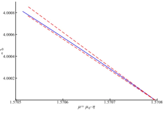
Figure 4: Narrow estimates on the period of the 0th branch of Example 3.3 by Theorem 9 (red dashed curves) compared to numerically obtained periods (blue solid curve).
In some situations this theorem provides very sharp estimations of the period function, which is illustrated in Figure 4.
Corollary 10. If in equation (1) the kth Hopf bifurcation is subcritical for some k≥0, and the periods satisfy Tηk< T0k near µk, then for alll≥1 the(k+l)th Hopf bifurcation is also subcritical.
Proof. If thekth Hopf bifurcation is subcritical, then
(µk−η)(lTηk+ 1)< µk(lT0k+ 1) =µk+l.
This means that the Cooke transformation maps thekth branch to the left side ofµk+l, thus the (k+l)th bifurcation is also subcritical.
In the situation H(0)B2 < C < H(∞)B2 (see Figure 2.b.), we can infer the monotonicity of the period functions at the subcritical bifurcations, as the next corollary shows.
Corollary 11. If in equation (1) thekth Hopf bifurcation is subcritical for somek≥0, but the(k+l)th Hopf bifurcation is supercritical for any l≥1, thenTηk >0 is monotone increasing for smallη.
Proof. If the kth Hopf bifurcation is subcritical, but the (k+l)th is supercritical, then for η1 < η2 we have
(µk−η1)(lTηk1+ 1)<(µk−η2)(lTηk2+ 1).
This is possible only ifTηk1 < Tηk2.
4.1 Application to Wright’s equation
There is a huge literature about the dynamics of equation (1) when f(ξ) = eξ −1, and the related conjectures of Wright and Jones (now proven theorems, see [1, 9]). In particular, Jaquette [9] has shown the following.
Theorem 12 (Jones’ conjecture). For every µ > π/2 there exists a unique slowly oscillating periodic solution to (2).
The 0th branch of (2) is formed by these unique slowly oscillating periodic solutions. The following conjecture is stated in [9, Conjecture 7.1].
Conjecture 13. The period length of slowly oscillating periodic solutions of (2)increases monotonically in µ.
The monotonicity was shown for µ ∈ (π/2, π/2 + 6.83×10⁻³] by Jaquette and van den Berg [1].
Applying our result, we can formulate the following theorem.
Theorem 14. The kth Hopf bifurcation branch of Wright’s equation (2) has no folds on the parameter interval (π/2 + 2kπ, π/2 + 2kπ+ 6.83×10⁻³(4k+ 1)], and the period length increases monotonically on this interval.
Proof. Fork= 0, we have the results of [1, 9], so there exists a unique periodic orbit on the 0th branch for each parameter value π/2 +η, η ∈(0,6.83×10−3]. Moreover, its period Tη0 is increasing in η, and Tη0→4 asη→0.
Letk ≥1. Using the Cooke transform Ck, as the 0th branch is mapped onto the kth branch, the parameterπ/2 +η is mapped toµ(η) = (π/2 +η)(kTη0+ 1). This is an increasing function ofηwith limit
η→0limµ(η) =π
2(4k+ 1) = π 2 + 2kπ.
UsingT6.83×100 −3 >4 (see [16]), we find from the Cooke transform that µ 6.83×10−3
=π
2 + 6.83×10⁻³
kT6.83×100 −3+ 1
≥ π
2 + 2kπ+ 6.83×10⁻³(4k+ 1).
Since the 0th branch has no fold on (π/2, π/2+6.83×10−3], and the Cooke transform maps this parameter interval monotone increasingly onto (π/2 + 2kπ, π/2 + 2kπ+ 6.83×10⁻³(4k+ 1)], thekth Hopf branch has no folds on this interval as well. The period on thekth branch for parameterµ(η) isTη0/(kTη0+ 1).
Choosing η1 andη2such that µ(η1), µ(η2)∈(π/2 + 2kπ, π/2 + 2kπ+ 6.83×10⁻³(4k+ 1)] andη1< η2, we have Tη01< Tη02 and
Tη0
2
kTη0
2+ 1− Tη0
1
kTη0
1+ 1 = kTη0
1Tη0
2+Tη0
2−kTη0
1Tη0
2−Tη0
1
(kTη0
1+ 1)(kTη0
2+ 1) = Tη0
2−Tη0
1
(kTη0
1+ 1)(kTη0
2+ 1) >0, hence the period is increasing along the kth branch as well.
Since Jones’ conjecture has been proven, it is now known that there are no folds on the 0th Hopf branch of slowly oscillating periodic solutions of Wright’s equation. Furthermore, isolas of slowly oscillating periodic solutions are excluded as well. By the Cooke transform, we can also exclude isolas of rapidly oscillatory periodic solutions. However, this is not sufficient to show there are no folds in the branches of rapidly oscillating periodic solutions [9]. Our Theorem 14 above shows the non-existence of folds on some intervals of the parameter on the Hopf branches of rapidly oscillatory solutions, using the monotonicity of the period established in [9] for a small interval of the 0th branch. Conjecture 13 would imply the absence of folds along all branches.
5 Schwarzian derivative and the direction of the Hopf bifurca- tion
The Schwarzian derivative of a C3 functionf is defined as (Sf)(ξ) = f000(ξ)
f0(ξ) −3 2
f00(ξ) f0(ξ)
2
at points ξwheref0(ξ)6= 0. This quantity plays an important role in many results regarding the global dynamics of difference equations, which can be extended to delay differential equations in various cases (see [11, 12, 13, 14] and references thereof). A global stability conjecture was formulated in [11], stating that the zero solution of (1) is globally asymptotically stable whenever it is locally asymptotically stable, Sf < 0, and some other technical conditions hold (for related conjectures, see [12]). An obvious way to disprove this global stability conjecture would be the following: find a nonlinearity f with Sf < 0, where the Hopf bifurcation of (1) is subcritical at µ0. This would provide a counterexample. Since both the directions of the bifurcation and the sign of the Schwarzian are determined by the derivatives of the nonlinearity up to order three, in view of the results of the previous sections, it is most natural to make a comparison to check whether the existence of such a counterexample is possible.
Corollary 15. If Sf < 0, then all Hopf bifurcations are supercritical. Furthermore, if f00(0) = 0, then for any k, the kth bifurcation is supercritical if and only ifSf(0)<0.
Proof. From the definition, it is easy to evaluateSf(0) = 6(C−B2), thusSf <0 impliesSf(0)<0 and C < B2. By Corollary 3, all Hopf bifurcations are supercritical. In the special casef00(0) = 0, we have B = 0 andSf(0) = 6C, thus both the sign of the Schwarzian and the direction of the bifurcation are determined by the sign of C.
We found that it is not possible to construct a counterexample to the conjecture of Liz et al. by means of a subcritical Hopf bifurcation.
Appendix
Proof of Theorem 1. a) The linearization of equation (1) is
x0(t) =−µx(t−1). (4)
From the exponential Ansatzx(t) =eλt, we get
λeλt=−µeλ(t−1), and the characteristic equation is
λ=−µe−λ.
To find the Hopf bifurcation points, we substituteλ=iω,ω∈R\ {0}, and write iω=−µe−iω=−µcosω+iµsinω.
Taking real and imaginary parts, we obtain the following system of real equations 0 =µcosω, ω=µsinω.
From the first equation, we get ω = π2 +nπ, n ∈Z. Substituting this into the second equation we
have π
2 +nπ =µsinπ 2 +nπ
. We distinguish two cases:
• n= 2k,k∈Z, in which case we find π
2 + 2kπ=µsinπ
2 + 2kπ
=µ;
• n= 2l+ 1,l∈Z, in which case we find π
2 + (2l+ 1)π=µsinπ
2 + (2l+ 1)π
=−µ, which is equivalent to
π
2 −(2l+ 2)π=µ.
We find that the viak =−(l+ 1), the two cases can be treated together, and for the critical values we may just writeµk = π2 + 2kπ= 4k+12 π, k∈Z. For eachµk there is a pair of critical eigenvalues
±iωk, where ωk =4k+12 π.
b) We follow the procedure developed in [4], using the parametrizationµ=µk+δkηas in Section 4. Let LandF be defined by the relation
L(δkη)xt+F(xt, δkη) =−(µk+δkη)f(x(t−1)),
where xt is the solution segment defined byxt(θ) =x(t+θ) forθ∈[−1,0]. Here,L(δkη) is a linear operator fromC([−1,0],R) toR,F is an operator fromC([−1,0],R)×RtoRwithF(0, δkη) = 0 and D1F(0, δkη) = 0. As equation (1) depends on the parameter linearly, we write
L(δkη) =L0+δkηL1, and, for (x1, x2, x3, x4)∈R4,
F(x1eiωkθ+x2e−iωkθ+x3·1 +x4e2iωkθ,0)
=B(2,0,0,0)x21+B(1,1,0,0)x1x2+B(1,0,1,0)x1x3+B(0,1,0,1)x2x4+B(2,1,0,0)x21x2+. . . Sinceµk =ωk= 4k+12 π, the equalityeiωk=iholds. Forφ∈C([−1,0],R) we have
L0(φ) =−µkφ(−1) =−4k+ 1
2 πφ(−1).
Hence,
L0(1) =−4k+ 1 2 π, L0(θeiωkθ) =−4k+ 1
2 π
−e−i4k+12 π
=−i4k+ 1 2 π, L0(e2iωkθ) =−4k+ 1
2 π
e−2i4k+12 π
=4k+ 1 2 π, and the expansion ofF can be written as
F(x1eiωkθ+x2e−iωkθ+x3·1 +x4e2iωkθ,0)
=−4k+ 1
2 π B(x1(−i) +x2i+x3−x4)2+C(x1(−i) +x2i+x3−x4)3+ h.o.t.
. Then theB(a,b,c,d)coefficients are
B(2,0,0,0)=4k+ 1
2 πB, B(1,1,0,0)=−(4k+ 1)πB, B(1,0,1,0)= (4k+ 1)πBi, B(0,1,0,1)= (4k+ 1)πBi, B(2,1,0,0)=3
2(4k+ 1)πCi.
According to [4] (see formula (3.18) and Theorem 3.20), the direction of the bifurcation is determined by the sign of
K= Re
1 1−L0(θeiωkθ)
B(2,1,0,0)−B(1,1,0,0)B(1,0,1,0)
L0(1) +B(2,0,0,0)B(0,1,0,1) 2iωk−L0(e2iωk)
.
We shall use the notationa∼bwhenevera=qbfor someq >0. Substituting all terms intoK, we need to find the sign of the real part of
1 1 +i4k+12 π
3
2(4k+ 1)πCi−−(4k+ 1)πB(4k+ 1)πBi
−4k+12 π +
4k+1
2 πB(4k+ 1)πBi i(4k+ 1)π−4k+12 π
!
=(2−(4k+ 1)πi) 2(1 +(4k+1)22 2)
(4k+ 1)π 3
2Ci−2B2i+(−2i−1)B2i 5
∼(2−(4k+ 1)πi)(4k+ 1) 3
2Ci+2
5B2−11 5 B2i
.
The latter expression has real part (4k+ 1)
(4k+ 1)π3 2C+4
5B2−11
5 (4k+ 1)πB2
∼C−H(k)B2.
c) To determine the direction a pair of characteristic roots crosses the imaginary axis at a bifurcation point, we differentiate the real part with respect to the parameter. Let us consider a parameter dependent solution of the characteristic equationλ=−µe−λ, written asλ(µ) =α(µ) +iω(µ), where αandω are the real and imaginary parts. Then we have
α+iω=−µe−α−iω=−µe−α(cosω−isinω).
Separating real and imaginary parts, we get
α=−µe−αcosω, ω=µe−αsinω.
Differentiating these equations with respect toµ, we find
α0=−e−αcosω−µe−α(−α0) cosω−µe−α(−sinω)ω0, ω0=e−αsinω+µe−α(−α0) sinω+µe−αcos(ω)ω0.
Assuming that the root is critical, α(µk) = 0 andω(µk) = ωk. As we have seen in part a), in the critical case cosωk = 0 and sinωk = 1. Then, evaluating the derivatives atµk, we obtain
α0=µkω0, ω0= 1−µkα0. Now we substituteω0 into the first equation, and expressα0 as
α0(µk) = µk
1 +µ2k.
Hence,α0(µk) andµkhas the same sign. This means that, at a Hopf bifurcation, a pair of characteristic roots crosses the imaginary axis from left to right if and only if µk > 0. Hence the branch of a supercritical Hopf bifurcation starts to the right if and only ifµk >0, and the subcritical case is the opposite.
Acknowledgements
IB was supported by the EU funded Hungarian project EFOP-3.6.2-16-2017-00015, 20391-3/2018/FEKUSTRAT and NKFI K129322. GR was supported by NKFI FK124016 and Marie Sk lodowska-Curie Grant No. 748193. The authors thank Maria Vittoria Barbarossa and Jan Sieber for helping with DDE-BifTool.
Compliance with ethical standards All authors declare that they have no conflict of interest.
References
[1] J. B. van den Berg, J. Jaquette: A proof of Wright’s conjecture.Journal of Differential Equations 264.12 (2018), pp. 7412–7462.
[2] S.-N. Chow, J. Mallet-Paret: Integral averaging and bifurcation.Journal of Differential Equations 26.1 (1977), pp. 112–159.
[3] O. Diekmann, S. A. van Gils, S. M. Verduyn Lunel, H.-O. Walther: Delay Equations. Springer (1995).
[4] T. Faria, L. T. Magalh˜aes: Normal Forms for Retarded Functional Differential Equations with Parameters and Applications to Hopf Bifurcation. Journal of Differential Equations 122.2 (1995), pp. 201–224.
[5] ´A. Garab, T. Krisztin: The period function of a delay differential equation and an applicatio.
Periodica Mathetmatica Hungarica 63.2 (2011), pp. 173–190.
[6] F. Giannakopoulos, A. Zapp: Local and Global Hopf Bifurcation in a Scalar Delay Differential Equation.Journal of Mathematical Analysis and Applications 237.2 (1999), pp. 425–450.
[7] S. Guo, J. Wu: Bifurcation Theory of Functional Differential Equations.Springer (2013).
[8] B. D. Hassard, N. D. Kazarinoff, Y-H. Wan: Theory and Applications of Hopf Bifurcation. Cam- bridge University Press (1981).
[9] J. Jaquette: A proof of Jones’ conjecture.Journal of Differential Equations 266.6 (2019), pp. 3818–
3859.
[10] B. Lani-Wayda: Hopf Bifurcation for Retarded Functional Differential Equations and for Semiflows in Banach Spaces.Journal of Dynamics and Differential Equations 25.4 (2013), pp. 1159–1199.
[11] E. Liz, M. Pinto, G. Robledo, S. Trofimchuk, V. Tkachenko: Wright Type Delay Differential Equa- tions with Negative Schwarzian.Discrete and Continuous Dynamical Systems 9.2 (2003), pp. 309–
321.
[12] E. Liz, G. R¨ost: Dichotomy results for delay differential equations with negative Schwarzian deriva- tive.Nonlinear Analysis: Real World Applications 11.3 (2010), pp. 1422–1430.
[13] E. Liz, G. R¨ost: On the Global Attractor of Delay Differential Equations with Unimodal Feedback.
Discrete and Continuous Dynamical Systems 24.4 (2009), pp. 1215–1224.
[14] E. Liz, G. R¨ost: Global dynamics in a commodity market model.Journal of Mathematical Analysis and Applications 398.2 (2013), pp. 707–714.
[15] J. Mallet-Paret, R. Nussbaum: Global continuation and asymptotic behaviour for periodic solutions of a differential-delay equation. Annali di Matematica Pura ed Applicata 145.1 (1986), pp. 33–128.
[16] R. Nussbaum: Wright’s equation has no solutions of period four.Proceedings of the Royal Society of Edinburgh 113.3–4 (1989), pp. 81–288.
[17] G. R¨ost: Bifurcation of Periodic Delay Differential Equations at Points of 1:4 Resonance. Func- tional Differential Equations 13.3–4 (2006), pp. 519–536.
[18] H. L. Smith: An Introduction to Delay Differential Equations with Applications to the Life Sciences.
Springer (2011).
[19] H. W. Stech: Hopf Bifurcation Calculations for Functional Differential Equations.Journal of Math- ematical Analysis and Applications 109.2 (1985), pp. 472–491.