Brain Tumor Segmentation from MRI Data Using Ensemble Learning and Multi-Atlas*

Brain Tumor Segmentation from MRI Data Using Ensemble Learning and Multi-Atlas*

T´ımea F¨ul¨op, ´Agnes Gy˝orfi, B´ela Sur´anyi, Levente Kov´acs and L´aszl´o Szil´agyi

Abstract— Atlases are frequently employed to assist med- ical image segmentation with prior information. This paper introduces a multi-atlas architecture that is trained to locally characterize the appearance (average intensity and standard deviation) of normal tissues in various observed and computed data channels of brain MRI records. The multiple atlas is then deployed to enhance the accuracy of an ensemble learning based brain tumor segmentation procedure that uses binary decision trees. The proposed method is validated using the low-grade tumor volumes of the BraTS 2016 train data set. The use of atlases improve the segmentation quality, causing a rise of up to 1.5% in average Dices scores.

Index Terms— Atlas-based image segmentation, multi-atlas, brain tumor segmentation, magnetic resonance imaging.

I. INTRODUCTION

Atlases and multi-atlases employed in medical image segmentation problems attempt to enhance the quality of the outcome using prior information regarding the object (organ) being segmented. Without atlases and shape models, segmen- tation methods can only use global and local properties of pixels (or voxels), like intensity distributions and textures.

The use of atlases enable us to add further information to the segmentation process, for example, what is usually present in the same place in other similar image records, or what intensities are usually present in the same place in other normal records.

Atlases have recently been involved in several medical imaging problems, including the segmentation of brain tis- sues and lesions [1], [2], [3], prostate [4], lung [5], cardiac structures (e.g. myocardium) [6], [7], pancreas [8], [9], bones [10], cartilage [11], and multiple abdominal organ [12]. Atlases are used in segmentation problems based on

*This project was supported in part by the Sapientia Institute for Research Programs. This project has received funding from the European Research Council (ERC) under the European Unions Horizon 2020 research and innovation programme (grant agreement No 679681). The work of T. F¨ul¨op was supported by the Collegium Talentum 2019 Programme of Hungary. The work of L. Szil´agyi was supported by the Hungarian Academy of Sciences through the J´anos Bolyai Fellowship program.

T. F¨ul¨op and B. Sur´anyi are with Dept. of Mathematics-Informatics, Sapientia University, Calea Sighis¸oarei 1/C, 540485 Tˆırgu Mures¸, Romania (phone: +40-265-206-210; fax: +40-265-206-211; e-mail:

{fuloptimea1427,bela.suranyi} at gmail.com).

A.´ Gy˝orfi, L. Kov´acs and L. Szil´agyi are with University Research, Innovation, and Service Center (EKIK), ´Obuda University, B´ecsi ´ut 96/b, H-1034 Budapest, Hungary (phone/fax: +36-1-666- 5585; e-mail: gyorfi.agnes at phd.uni-obuda.hu, {kovacs.levente, szilagyi.laszlo} at

nik.uni-obuda.hu).

A. Gy˝orfi and L. Szil´agyi are also with Dept. of Electrical En-´ gineering, Sapientia University, Calea Sighis¸oarei 1/C, 540485 Tˆırgu Mures¸, Romania (phone: +40-265-206-210; fax: +40-265-206-211; e-mail:

{gyorfiagnes,lalo} at ms.sapientia.ro).

image data originating from virtually all imaging modalities, including magnetic resonance images (MRI) [1], [2], [4], computed tomography (CT) [5], [9], [10], CT angiography [6], positron emission tomography (PET) [7], X-ray [13] and mammography [14]. A systematic review of earlier image segmentation solutions based on atlases and multi-atlases is given by Cabezas et al. [15]. Several earlier atlas-based solutions are summarized in the review paper of Gordillo et al. [16]. A more recent summary of such methods can be found in the work of Sun et al.[17].

This paper proposes an atlas-based extension for a brain tumor segmentation procedure that uses ensemble learning with binary decision trees. Multiple atlases are built, one for each feature, using only the normal voxels of the train data. The atlases will be able to say, what is the normal average intensity and the standard deviation of intensities at any position within the volume. These atlas values are used to update all feature values before proceeding to the training and testing of the decision tree ensemble. Numerical experi- ments will be performed to show the benefits brought by the multi-atlas approach, and to establish the best parameters of the atlas.

The rest of this paper is structured as follows: Section II presents the proposed segmentation method with full details on how the atlases are built and applied. Section III describes the experimental validation of the proposed methods. Section IV concludes the study.

II. MATERIALS AND METHODS

We start from an existing brain tumor segmentation pro- cedure [18], [19], which is based on ensemble learning using binary decision trees (BDT) [20]. The BDTs are trained to separate voxels belonging to focal lesions from those that represent normal brain tissues. The separation relies on four observed and 100 computed features. The accuracy of the segmentation is evaluated statistically, the main accuracy indicator being the Dice score, which penalised the misclassi- fication of both positive and negative voxels. The main goal of this study is to prove that adding prior information to the segmentation procedure using atlases can improve the accuracy of segmentation.

A. Data

The MICCAI Brats 2016 train data set contains 220 high- grade (HG) and 54 low-grade (LG) tumor volumes [21]. This study uses the whole set of LG tumor data. All volumes have the same size, consisting of 155 slices, each of which contain 240×240 voxels. Each record contains four data

channels (T1, T2, T1C, FLAIR) that represent the observed features for all voxels. Each voxel has a label established by human experts, which is used as ground truth in our study.

All data channels were registered to the T1 data using a standard automatic method and all other non-brain tissues were removed from all volumes [21]. LG tumor volumes were randomly divided in two equal groups. These groups took turns in serving as train and test data.

B. The segmentation procedure without atlas

The tumor segmentation procedure we start from was previously described in details in our previous paper [18].

MRI volumes were processed in several steps as listed below:

1) The first step is the so-called preprocessing, which is composed of the following tasks: (1) compensation of intensity inhomogeneity [22], [23], [24] using an enhanced N3 method [25]; (2) histogram normalization to provide comparable intensities on all data channels within the interval[α₀, β₀], accomplished by a context sensitive linear transform whose details are given in our previous work [26].

2) The expected correlation between neighbor voxels, and the imperfection of the automatic registration processes applied to align the four observed data channels mo- tivate the feature generation that follows the prepro- cessing. Feature generation equally applies to all four observed data channels. Generated features include:

(1) average, minimum and maximum extracted from spatial3×3×3-sized neighborhood; (2) average and median values extracted from planar neighborhoods with sizes ranging from3×3 to11×11; (3) gradient values extracted from7×7-sized neighborhood in four different directions; (4) Gabor wavelet values extracted from 11×11-sized neighborhood in eight different directions. Together with the four observed ones, the total number of features becomesN_ϕ= 104.

3) An ensemble learning approach is employed to ac- complish the classification of voxels, built from binary decision trees. A number of nT = 125 decision trees are trained to separate normal and tumor voxels of the train data set. Each tree is trained using N randomly selected voxels of the train data, out of which pN = 93% are negatives. The procedure was tested with values of parameterN ranging from 10 thousand (10k) to one million (1000k). Each non-leaf node of the decisions trees learns to make an optimal decision comparing a certain feature with a threshold, which were established by entropy based criterion. During the ensemble testing, each voxel of the test dataset receives a vote from each decision tree of the ensemble. The majority of the votes define the intermediary labeling of the test voxels.

4) Post-processing reevaluates the intermediary label of each test voxel using a morphological criterion: it com- pares the rate of positive intermediary voxels within a 11×11×11 neighborhood of the current voxel with a previously defined threshold. Voxels with frequent

positive neighbors are declared positive, regardless to the own intermediary labeling. Post-processing leads to regularized tumor shapes and improved accuracy indicator values.

C. The multi-atlas approach

Let us denote the whole set of MRI volumes involved in this study by Γ, the set of train volumes by Γ⁽¹⁾, and the set of test volumes byΓ⁽²⁾. Obviously,Γ = Γ⁽¹⁾∪Γ⁽²⁾, and Γ⁽¹⁾∩Γ⁽²⁾= Φ. Further on,Ω⁽¹⁾_i will stand for theith train volume, i = 1. . .|Γ⁽¹⁾|, which contains |Ω⁽¹⁾_i | voxels with intensities ω_ik⁽¹⁾ ∈ [α₀, β₀], k = 1. . .|Ω⁽¹⁾_i |. Analogously, Ω⁽²⁾_j will stand for the jth test volume, j = 1. . .|Γ⁽²⁾|, which contains|Ω⁽²⁾_j |voxels with intensitiesω⁽²⁾_jk ∈[α₀, β₀], k = 1. . .|Ω⁽²⁾_j |. Let us further denote by N the set of all voxels that are negative by grand truth.

In this study we propose and evaluate a multi-atlas ap- proach that provides additional local information to each of the observed and computed features. In this order, for each feature we build an atlas based on the intensity values of normal voxels of the train data set. An important parameter that controls the size of the atlases is denoted by S. The proposed method was evaluated for various values of this parameter, ranging from 60 to 120. In fact, the atlas built for any of the 104 features represents a 3-dimensional array of size (2S+ 1)×(2S+ 1)×(2S+ 1). Let us denote the set of possible atlas coordinates in any of the three main directions by S, so S ={−S,−S+ 1, . . .0. . . , S−1, S}.

The atlas for feature number ϕ (ϕ = 1. . . N_ϕ) will be a function Aϕ : S³ → R³, which for any point Pˆ ∈ S³ situated at coordinates(ˆx,y,ˆ ˆz)gives the triple(ˆµPˆ,σˆPˆ,νˆPˆ) which represent an average intensity, a standard deviation of intensities, and the number of values used to compute the previous two, respectively.

One more definition is needed before explaining the atlas building process. For any atlas point Pˆ of coordinates (ˆx,y,ˆ z)ˆ we define its cubic neighborhood

Cδ( ˆP) ={( ˆα,β,ˆ γ)ˆ ∈ S³,|αˆ−x| ≤ˆ δ ∧

∧ |βˆ−y| ≤ˆ δ ∧ |ˆγ−z| ≤ˆ δ} , (1) whereδis a small positive integer, typically one ore two.

We need to define a function for each volume that maps it onto the atlas. For the ith train volumeΩ⁽¹⁾_i , this function is defined as fi : V → S³, where V describes the definition domain of the original volumes,V = [0. . .239]× [0. . .239]×[0. . .154]. We will use these mapping functions to find the corresponding atlas position for all brain pixels.

To build these mapping functions we need to compute the following:





 µ⁽ⁱ⁾x

µ⁽ⁱ⁾y

µ⁽ⁱ⁾z





= 1

|Ω⁽¹⁾_i | X

(x,y,z)∈Ω⁽¹⁾_i



 x y z



 , (2)

Algorithm 1: Build the atlas function Aϕ for each feature ϕ= 1. . . Nϕ and apply to all feature data

Data:Set of MRI volumes involved in the study Γ, each with Nϕ extracted features.

Data:Parameters S andδ

Result:Atlas functions Aϕ,ϕ= 1. . . Nϕ

Define set of train and test volumes, Γ⁽¹⁾ andΓ⁽²⁾. fori= 1. . .|Γ⁽¹⁾|do

Compute the mapping function f_i(π)for every voxelπ∈Ω⁽¹⁾_i using Eqs. (2)-(4).

end

forj = 1. . .|Γ⁽²⁾|do

Compute the mapping function gj(π)for every voxelπ∈Ω⁽²⁾_j using Eqs. (2)-(4).

end

forϕ= 1. . . N_ϕ do

Compute the atlas function Aϕ( ˆP)for every discrete point Pˆ ∈ S³ using Eqs. (5)-(9).

fori= 1. . .|Γ⁽¹⁾|do

Update the intensity at feature ϕfor every voxel π∈Ω⁽¹⁾_i with the value given in Eq. (10).

end

forj = 1. . .|Γ⁽²⁾|do

Update the intensity at feature ϕfor every voxel π∈Ω⁽²⁾_j with the value given in Eq. (11).

end end





 σx⁽ⁱ⁾

σy⁽ⁱ⁾

σz⁽ⁱ⁾





=



























 v u u t

P

(x,y,z)∈Ω(1) i

x−µ⁽ⁱ⁾x

2

|Ω⁽¹⁾_i |−1

v u u t

P

(x,y,z)∈Ω(1) i

y−µ⁽ⁱ⁾y

2

|Ω⁽¹⁾_i |−1

v u u t

P

(x,y,z)∈Ω(1) i

z−µ⁽ⁱ⁾z

2

|Ω⁽¹⁾_i |−1





























. (3)

The mapping is finally defined as

fi(x, y, z) =

















S(x−µ⁽ⁱ⁾_x )

ξσ⁽ⁱ⁾_x

S(y−µ⁽ⁱ⁾_y )

ξσ⁽ⁱ⁾_y

S(y−µ⁽ⁱ⁾_z )

ξσ⁽ⁱ⁾_z

















T

, (4)

whereξ = 2.5 is a scaling factor, and hqi is the value of floating point variableq rounded to the closest integer.

In an analogous way, we build similar mapping functions g_j : V → S³, for every test volume with index j = 1. . .|Γ⁽²⁾|.

The atlas function for feature ϕhas the form Aϕ( ˆP) = ˆµPˆ,σˆPˆ,ˆνPˆ

, (5)

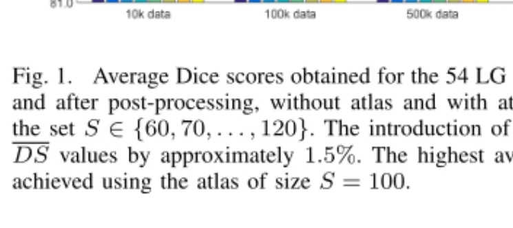
Fig. 1. Average Dice scores obtained for the 54 LG tumor volumes, before and after post-processing, without atlas and with atlas of size ranging in the setS∈ {60,70, . . . ,120}. The introduction of the atlas improves all DS values by approximately 1.5%. The highest average Dice scores are achieved using the atlas of sizeS= 100.

which for any Pˆ ∈ S³ is established with the following formulas:

ˆ ν_Pˆ=

|Γ⁽¹⁾|

X

i=1

X

π∈Ψ⁽¹⁾

i,Pˆ

1 , (6)

ˆ

µPˆ = 1 ˆ ν( ˆP)

|Γ⁽¹⁾|

X

i=1

X

π∈Ψ⁽¹⁾

i,Pˆ

ω⁽¹⁾_iπ , (7)

ˆ σPˆ=

v u u u u u t

|Γ⁽¹⁾|

P

i=1

P

π∈Ψ⁽¹⁾

i,Pˆ

ω⁽¹⁾_iπ −µˆ_Pˆ²

ˆ

ν_Pˆ−1 , (8)

where Ψ⁽¹⁾

i,Pˆ ={p∈Ω⁽¹⁾_i , fi(p)∈ Cδ( ˆP)∧ Ω⁽¹⁾_i (π)∈ N } . (9) The intensity values of each voxel π ∈ Ω⁽¹⁾_i (i = 1. . .|Γ⁽¹⁾|) in the train data set, denoted byω⁽¹⁾_iπ, is updated with the value given by the formula:

min (

max (

α0,

*

µ+σω⁽¹⁾_iπ −µ(fˆ i(π)) ˆ

σ(fi(π)) +)

, β0

) . (10) Recommended parameter values are µ = (α₀+β₀)/2 and σ= (β₀−α₀)/10.

The intensity values of each voxel π ∈ Ω⁽²⁾_j (j = 1. . .|Γ⁽²⁾|) in the test data set, denoted byω_jπ⁽²⁾, is updated according to the atlas functions created for the train data set, with value given by the formula:

min (

max (

α₀,

*

µ+σω_jπ⁽²⁾−µ(gˆ _j(π)) ˆ

σ(gj(π)) +)

, β₀ )

. (11) Updated intensity values for all voxels and all features are fed to the very same training and testing process presented in Section II-B.

The whole process of construction and usage of the multi- atlas is summarized in Algorithm 1.

TABLE I

AVERAGE VALUES OF ACCURACY INDICATORS IN CASE OF VARIOUS SIZES OF THE TRAIN DATA SET,OBTAINED WITH NO ATLAS OR WITH ATLAS OF DIFFERENT SIZES.

Accuracy Data Atlas size

indicator size no atlas S= 60 S= 70 S= 80 S= 90 S= 100 S= 110 S= 120

10k 81.458 82.159 82.278 82.200 82.333 82.326 82.288 82.160

Average 100k 82.519 82.926 82.975 83.020 83.048 83.062 83.033 82.964

Dice score 500k 82.473 83.187 83.241 83.253 83.336 83.352 83.290 83.223

1000k 82.480 83.203 83.270 83.250 83.348 83.354 83.313 83.221

10k 83.526 83.993 84.101 84.045 84.169 84.173 84.115 84.004

Overall 100k 84.320 84.584 84.605 84.642 84.673 84.688 84.649 84.563

Dice score 500k 84.322 84.721 84.774 84.764 84.857 84.873 84.818 84.731

1000k 84.346 84.784 84.808 84.774 84.864 84.881 84.830 84.740

10k 83.480 83.432 83.598 83.365 83.431 83.466 83.507 83.263

Average 100k 85.332 84.967 85.005 84.884 84.987 85.034 84.978 84.813

Sensitivity 500k 86.266 85.760 85.846 85.695 85.907 85.957 85.831 85.688

1000k 86.860 86.265 86.351 86.224 86.400 86.454 86.380 86.179

10k 98.775 98.832 98.832 98.844 98.857 98.854 98.840 98.848

Average 100k 98.733 98.774 98.773 98.792 98.786 98.782 98.782 98.787

Specificity 500k 98.638 98.715 98.715 98.731 98.723 98.719 98.724 98.725

1000k 98.575 98.669 98.670 98.677 98.675 98.669 98.670 98.677

Fig. 2. Average Sensitivity values obtained for the 54 LG tumor volumes, before and after post-processing, without atlas and with atlas of size ranging in the setS ∈ {60,70, . . . ,120}. Post-processing improves all average Sensitivity values by approximately10%, however, the atlases seem to slightly damage this improvement.

Fig. 3. Average Specificity values obtained for the 54 LG tumor volumes, before and after post-processing, without atlas and with atlas of size ranging in the set S ∈ {60,70, . . . ,120}. Atlases seem to contribute to the improvement of average Specificity values by approximately0.1%.

D. Evaluation

Segmentation accuracy of volumeΩ⁽²⁾_j (j = 1. . .|Γ⁽²⁾|) is described by the number of true positive (TP_j), false positive (FPj), true negative (TNj) and false negative (FNj) voxels.

The most important accuracy indicators for an arbitrary test volumeΩ⁽²⁾_j (j= 1. . .|Γ⁽²⁾|) are:

1) Sensitivity (also referred to as true positive rate, TPR) represents the rate of identified positives among all

positive voxels, and thus penalizes the occurrence of false negatives:

TPR_j= TP_j TPj+ FNj

. (12)

2) Specificity (also referred to as true negative rate, TNR) represents the rate of identified negatives among all negative voxels, and thus penalizes the occurrence of false positives:

TNR_j = TNj

TN_j+ FP_j . (13) 3) The Dice Score (DS) is our main accuracy indicator, which penalizes the occurrence of both false positives and false negatives:

DSj= 2×TPj

2×TP_j+ FP_j+ FN_j . (14) The average Dice score is the mean of the Dice scores obtained for individual volumes and is computed with the formula

DS = 1

|Γ⁽²⁾|

|Γ⁽²⁾|

X

j=1

DSj , (15)

while the overall Dice score treats the test data set as a whole, and thus is defined as

DS =f

2×

|Γ⁽²⁾|

P

j=1

TPj

|Γ⁽²⁾|

P

j=1

(2×TP_j+ FP_j+ FN_j)

. (16)

Similarly, it is possible to extract average and overall values for sensitivity and specificity as well.

Swapping the role of the two sets Γ⁽¹⁾ and Γ⁽²⁾ allows us to have segmentation accuracy indicators for all available MRI volumes.

Fig. 4. Dice scores obtained for individual LG tumor volumes with no atlas. The trees of the ensemble were trained with feature vectors of 500k voxels.

Fig. 5. Dice scores obtained for individual LG tumor volumes with the atlas of sizeS= 100. The trees of the ensemble were trained with feature vectors of 500k voxels.

III. RESULTS AND DISCUSSION

The whole set of 54 LG tumor volumes was divided into two disjoint set of records, each of which played the role of train and test data set in turns. In each turn, atlases of various sizes were built using values of parameterSranging from 60 to 120 in steps of 10, while parameterδwas set to one. Ensembles were trained using feature vector sets ranging from ten thousand to one million items, out of which 93%

were negatives and 7% positives. The training and testing cycle was performed for all cases and accuracy indicators recorded for each volume separately. Statistical evaluation was performed based on these recorded accuracy indicator values.

Fig. 6. Expected Dice scores for tumors of10cm³and100cm³computed with linear regression, at various sizes of the train data set. The atlas used here is the one with sizeS= 100. The atlas improves Dice scores by2%

in case of small tumors and by1%case of large tumors.

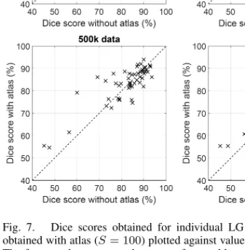
Fig. 7. Dice scores obtained for individual LG tumor volumes, values obtained with atlas (S= 100) plotted against values obtained without atlas.

The four graphs represent the cases of ensembles whose trees were trained with 10k, 100k, 500k, and 1000k feature vectors, respectively. Average Dice score is higher when the atlas is used, but individual values can be lower.

Table I reports average and overall values of the most important accuracy indicators obtained over the whole LG tumor volumes, in all the scenarios depicted in the previous paragraph. Highest indicator values are highlighted in each row of the table. Dice scores are at their highest when using the S = 100 atlas. Sensitivity and specificity values by themselves only show that using the atlas yields the pre- diction of more positives, but Dice scores become definitely higher by0.5−1.0%. Figures 1, 2, and 3 exhibit the same average accuracy indicator values in graphical representation, before and after post-processing. These graphs reveal further phenomena:

1) larger train data sets provide higher DS and TPR values, and lower TNR values;

2) TPR values become higher at the ensemble output when we use the atlas, but not after post-processing, suggesting the need for an intelligent, machine learning based post-processing instead of the currently used morphological one;

3) the beneficial effect of the atlas seems to be at its highest at90≤S≤100.

Linear regression was employed to establish the trend of Dice scores obtained for individual LG tumor volumes, without using atlas and with using the best performing atlas.

Figures 4, 5 and 6 exhibit the main findings. Figure 4 plots the obtained individual Dice scores against the true size of the tumor, and indicates the detected linear trend with the dashed line, for the no atlas case. Figure 4 plots the same thing in case of atlas usage. The difference is best visible for smaller tumors: using the atlas increases the expected Dice

score by 1.5%, it is well over80% while it was below that when no atlas was employed. Figure 6 shows the effect of the atlas according to the linear trend for two selected sizes of the tumor, in case of various sizes of the ensemble training data set. Trends predict a1.0−1.5%and0.7−1.0%increase of the Dice score for a10cm³and a100cm³-volume tumor, respectively.

Figure 7 shows the effect of the atlas upon Dice scores obtained for individual LG tumor volumes, plotting DS values achieved with atlas (S = 100) against DS values achieved without atlas. The four graphs exhibit the cases of different train data sizes, from 10k to 1000k feature vectors for each decision tree of the ensemble. These graphs also indicate that the beneficial effect of the atlas is better visible in case of lower Dice score achieved without atlas. The use of the atlas improves the average quality of segmentation, but there are several MRI records which get higher Dice scores without atlas.

The average accuracy of the proposed atlas-based method is at the median level of deep neural network based solutions that competed at the BraTS 2017 and 2018 challenges [27].

However, our method was tested on LG volumes of the BraTS 2016 challenge only.

IV. CONCLUSIONS

This paper introduced an ensemble learning based brain tumor segmentation algorithm enhanced by multiple atlases.

An atlas was built for each feature, locally representing the average intensity of normal voxels of the train data set, together with the standard deviation of intensities. Feature values of every voxel in the train and test data set were updated using a formula that involves the extracted atlases.

The updated feature values underwent the same ensemble training and testing process. Numerical evaluation revealed that the use of atlases improves the average segmentation accuracy by1.0−1.5%.

REFERENCES

[1] Y. Y. Yang, W. J. Jia and Y. N. Yang, “Multi-atlas segmentation and correction model with level set formulation for 3D brain MR images,”

Patt. Recogn., vol. 90, pp. 450–463, 2019.

[2] S. X. Bao, C. Bermudez, Y. K. Huo, P. Parvathaneni, W. Rodriguez, S. M. Resnick, P. F. D’Haese, M. McHugo, S. Heckers, B. M. Dawant, I. Lyu and B. A. Landman, “Registration-based image enhancement improves multi-atlas segmentation of the thalamic nuclei and hip- pocampal subfields,”Magn. Res. Imag., vol. 59, pp. 143–152, 2019.

[3] J. Huo, J. Wu, J. W. Cao and G. H. Wang, “Supervoxel based method for multi-atlas segmentation of brain MR images,”NeuroImage, vol.

175, pp. 201–214, 2018.

[4] H. J. Jia, Y. Xia, Y. Song, W. D. Cai, M. Fulham and D. D. Feng,

“Atlas registration and ensemble deep convolutional neural network- based prostate segmentation using magnetic resonance imaging,”Neu- rocomput., vol. 280, pp. 1358–1369, 2018.

[5] J. H. Zhou, Z. N. Yan, G. Lasio, J. Z. Huang, B. S. Zhang, N.

Sharma, K. Prado and W. D’Souza, “Automated compromised right lung segmentation method using a robust atlas-based active volume model with sparse shape composition prior in CT ,”Comput. Med.

Imag. Graph., vol. 46, pp. 47–55, 2015.

[6] Y. M. Niu, Q. Lan and X. C. Wang, “Structured graph regularized shape prior and cross-entropy induced active contour model for myocardium segmentation in CTA images,”Neurocomput., vol. 357, pp. 215–230, 2019.

[7] S. J. W. Kim, S. Seo, H. S. Kim, D. Y. Kim, K. W. Kang, J. J. Min and J. S. Lee, “Multi-atlas cardiac PET segmentation,”Phys. Med., vol. 58, pp. 32–39, 2019.

[8] K. Karasawa, M. Oda, T. Kitasaka, K. Misawa, M. Fujiwara, G. W.

Chu, G. Y. Zheng, D. Rueckert and K. Mori, “Multi-atlas pancreas segmentation: Atlas selection based on vessel structure,”Med. Image Anal., vol. 39, pp. 18–28, 2017.

[9] O. Acosta, E. Mylona, M. Le Dain, C. Voisin, T. Lizee, B. Rigaud, C. Lafond, K. Gnep and R. De Crevoisier, “Multi-atlas-based seg- mentation of prostatic urethra from planning CTimaging to quantify dose distribution in prostate cancer radiotherapy,”Radiotherapy and Oncology, vol. 125, pp. 492–499, 2017.

[10] H. Arabi and H. Zaidi, “Comparison of atlas-based techniques for whole-body bone segmentation,”Med. Image Anal., vol. 36, pp. 98–

112, 2017.

[11] L. Shan, C. Zach, C. Charles and M. Niethammer, “Automatic atlas- based three-label cartilage segmentation from MR knee images,”Med.

Image Anal., vol. 18, pp. 1233–1246, 2014.

[12] B. Oliveira, S. Queir´os, P. Morais, H. R. Torres, J. Gomes-Fonseca, J. C. Fonseca and J. Vilac¸a, “A novel multi-atlas strategy with dense deformation field reconstruction for abdominal and thoracic multi- organ segmentation from computed tomography,”Med. Image Anal., vol. 45, pp. 108–120, 2018.

[13] D. C. T. Nguyen, S. Benameur, M. Mignotte and F. Lavoie, “Super- pixel and multi-atlas based fusion entropic model for the segmentation of X-ray images,”Med. Image Anal., vol. 48, pp. 58–74, 2019.

[14] M. K. Sharma, M. Jas, V. Karale, A. Sadhu and S. Mukhopadhyay,

“Mammogram segmentation using multi-atlas deformable registra- tion,”Comput. Biol. Med, vol. 110, pp. 244–253, 2019.

[15] M. Cabezas, A. Oliver, X. Llad´o, J. Freixenet and M. Bach Cuadra,

“A review of atlas-based segmentation for magnetic resonance brain images,”Comput. Meth. Prog. Bio., vol. 104, pp. e158–e177, 2011.

[16] N. Gordillo, E. Montseny and P. Sobrevilla, “State of the art survey on MRI brain tumor segmentation,”Magn. Reson. Imaging, vol. 31, pp. 1426–1438, 2013.

[17] L. Sun, L. Zhang and D. Q. Zhang, “Multi-atlas based methods in brain MR image segmentation,”Chin. Med. Sci. J., vol. 34, no. 2, pp.

110–119, 2019.

[18] L. Szil´agyi, D. Icl˘anzan, Z. Kap´as, Zs. Szab´o, ´A. Gy˝orfi and L.

Lefkovits, “Low and high grade glioma segmentation in multispectral brain MRI data”,Acta Universitatis Sapientiae, Informatica, vol. 10, no. 1, pp. 110–132, 2018.

[19] Zs. Szab´o, Z. Kap´as, ´A. Gy˝orfi, L. Lefkovits, S. M. Szil´agyi and L.

Szil´agyi, “Automatic segmentation of low-grade brain tumor using a random forest classifier and Gabor features”,Proc. 14th International Conference on Fuzzy Systems and Knowledge Discovery, Huangshan, China, 2018, pp. 1106–1113.

[20] S. B. Akers, “Binary decision diagrams,” IEEE Transactions on Computers, vol. C-27, pp. 509–516, 1978.

[21] B. H. Menze, A. Jakab, S. Bauer, J. Kalpathy-Cramer, K. Farahani, J. Kirby et al., “The multimodal brain tumor image segmentation benchmark (BRATS),”IEEE Trans. Med. Imag., vol. 34, pp. 1993–

2024, 2015.

[22] U. Vovk, F. Pernu˘s and B. Likar, “A review of methods for correction of intensity inhomogeneity in MRI,”IEEE Trans. Med. Imag., vol. 26, pp. 405–421, 2007.

[23] L. Szil´agyi, S. M. Szil´agyi, B. Beny´o and Z. Beny´o, “Intensity inhomogeneity compensation and segmentation of MR brain images using hybridc-means clustering models”,Biomed. Sign. Proc. Contr., vol. 6, no. 1, pp. 3–12, 2011.

[24] L. Szil´agyi, S. M. Szil´agyi, and B. Beny´o, “Efficient inhomogeneity compensation using fuzzyc-means clustering models”,Comput. Meth.

Progr. Biomed, vol. 108, no. 1, pp. 80–89, 2012.

[25] N. J. Tustison, B. B. Avants, P. A. Cook, Y. J. Zheng, A. Egan, P.

A. Yushkevich and J. C. Gee, “N4ITK: improved N3 bias correction,”

IEEE Trans. Med. Imag., vol. 29, no. 6, pp. 1310–1320, 2010.

[26] ´A. Gy˝orfi, Z. Karetka-Mezei, D. Icl˘anzan, L. Kov´acs and L.

Szil´agyi,“A study on histogram normalization for brain tumour seg- mentation from multispectral MR image data,”Proc. Ibero-American Congress on Pattern Recognition (CIARP 2019, Havana), Lecture Notes in Computer Science, vol. 11896, pp. 375–384, 2019.

[27] S. Bakas, M. Reyes, A. Jakab, S. Bauer, M. Rempfler, A. Crimi et al., “Identifying the best machine learning algorithms for brain tumor segmentation, progression assessment, and overall survival prediction in the BRATS challenge,” arXiv: 1181.02629v2, 19 Mar 2019.