Research Article
Dynamic Modeling of the Angiogenic Switch and Its Inhibition by Bevacizumab
Dávid Csercsik
1,2and Levente Kovács
11Physiological Controls Research Center, University Research, Innovation and Service Center, ´Obuda University, Budapest, Hungary
2P´azm´any P´eter Catholic University, Faculty of Information Technology and Bionics, P.O. Box 278, 1444 Budapest, Hungary
Correspondence should be addressed to D´avid Csercsik; csercsik@itk.ppke.hu
Received 10 September 2018; Revised 12 November 2018; Accepted 12 December 2018; Published 3 January 2019
Guest Editor: Alejandro F. Villaverde
Copyright © 2019 D´avid Csercsik and Levente Kov´acs. This is an open access article distributed under the Creative Commons Attribution License, which permits unrestricted use, distribution, and reproduction in any medium, provided the original work is properly cited.
We formulate a dynamic model of vascular tumor growth, in which the interdependence of vascular dynamics with tumor volume is considered. The model describes the angiogenic switch; thus the inhibition of the vascularization process by antiangiogenic drugs may be taken into account explicitly. We validate the model against volume measurement data originating from experiments on mice and analyze the model behavior assuming different inputs corresponding to different therapies. Furthermore, we show that a simple extension of the model is capable of considering cytotoxic and antiangiogenic drugs as inputs simultaneously in qualitatively different ways.
1. Introduction
Neovascularization means the formation of new blood ves- sels. Angiogenesis, an important form of neovascularization, is characterized by hypoxia-driven sprouting of new capil- laries from postcapillary venules. This mechanism plays an important role in many physiological (e.g., wound healing [1]) and pathological (e.g., macular degeneration [2]) pro- cesses. In the development of tumors, angiogenesis plays an exceptionally important role [3, 4]. In the beginning, when the tumorous cells form a small plaque, the tumor cells are well supported with metabolites by diffusion from the environment. However, as the size of the tumor increases, cells in the inside become insufficiently supported. Tumor- induced angiogenesis is the process of blood vessel formation, in which new vasculature is formed in order to support these insufficiently supported tumor cells.
Lately, much has been revealed about the details of tumor- induced angiogenesis and the underlying biochemical and biomechanical regulatory processes. These studies served as basis for the development of targeted molecular therapies [5]. The aim of these therapies is to inhibit tumor-related angiogenesis, thus cutting the tumor from metabolic support.
Bevacizumab (Avastin) is a pharmacotherapeutic antian- giogenic agent developed to withhold pathological angiogen- esis [6] via the inhibition of the tumor angiogenic factor VEGF (vascular endothelial growth factor) [7]. VEGF may be considered as a representative member of the family of biochemical agents promoting angiogenesis, called tumor angiogenic factors (TAFs).
In [8], two different dosage protocols of bevacizumab were compared. In the case of the first protocol, experimental animals (mice) received one high dose according to the generally accepted medical principle, while in the case of the second protocol (quasi-continuous therapy), a much lower dose was delivered every day of the therapy. Results have shown that the quasi-continuous protocol was more effective, while the total injected amount of the drug was significantly less. As antiangiogenic agents are expensive, the total used drug amount is an important aspect to consider in therapeutic design. In addition, reduction of therapeutic doses is also desirable to minimize drug side effects. The result described in [8] underlines the importance of therapy optimization in the case of the application of antiangiogenic drugs and shows that computational methods may help to exploit the potentials of this approach.
Volume 2019, Article ID 9079104, 18 pages https://doi.org/10.1155/2019/9079104
On the other hand, based on the new data and paradigms brought to light in biological studies on angiogenesis, compu- tational modeling of tumor-related vasculature development has became popular in the last decades, producing numerous computational models describing tumor growth and tumor- induced angiogenesis under different physiological circum- stances (for a review on mathematical modeling of angio- genesis, see [9–12], while for a biological viewpoint on the mechanisms of physiological and tumor-related/pathological angiogenesis, one may refer to [13]). An important aspect of these modeling studies is to predict the effect of possible therapeutic approaches in cancer treatment [14–16].
A large part of the aforementioned models exhibit a quite high level of complexity, which implies that while they may be potentially appropriate for the comparison of different therapeutic approaches under the assumption of a given parameter set, it can be challenging to fit them to single patients. Furthermore, exact therapy optimization may be computationally infeasible if one relies on complex and spatially detailed models as [17, 18].
Feedback control [19, 20] may be an alternative to offline therapy optimization approaches. One benefit of closed- loop methods is that, assuming appropriate physiological signals, they may provide performance guarantees also in the presence of parametric uncertainties [21]. Other potential benefits of closed-loop treatments over protocol-based can- cer therapies are discussed in [22]. In the case of diabetes, a similar biological control problem, such approaches have been successfully applied [23–27]. Control theoretic meth- ods require, however, concentrated parameter models and ordinary differential (or difference) equation models with moderate complexity to perform well.
Recently, a simple dynamical model of tumor growth and the effect of the antiangiogenic drug bevacizumab has been published [28]. This model contains very few parameters and state variables and thus it is ideal for parameter estimation and controller design purposes. This model is based on three state variables, namely, the proliferating tumor volume, the necrotic tumor volume, and the concentration of the angio- genic inhibitor. Although this model provides a good fit for certain experimental data (see the data later in Section 2.2), it holds some flaws.
First, as it does not include the description of vasculature dynamics, its drawback is that it is unable to interpret advanced measurement data corresponding to tumor and vasculature evolution dynamics, potentially available in the foreseeable future. Recently, several imaging techniques have been described, which allow the reconstruction of vascular microstructures: Doppler optical frequency domain imaging [29] and functional photoacoustic microscopy [30] are used today already in in vivo setups to map vascular networks, while diffusible iodine-based contrast-enhanced computed tomography [31] may be used in terminal experimental animals. These methods could provide valuable data about vasculature dynamics in the near future, which may be used for the identification of the details of the angiogenic processes.
Second, minimal models not including vasculature dynamics as [28] are lacking the potential to describe the
phenomenon of the angiogenic switch [32]. This hypothesis, formulated by Folkman, assumes that angiogenesis begins only at a certain stage of tumor development, more precisely at the time when the limited diffusion distance (which is about 0.1 mm [33]) makes the support of tumor cells inside the tumor with oxygen and metabolites no longer possible.
According to the prediction of the minimal model [28], antiangiogenic drugs significantly affect the tumor growth also in the initial period. This contradicts with the consid- eration based on Folkman’s hypothesis that implies that in the initial period no insufficiently supported tumor cells are present, so no TAF synthesis is present; thus its effect can not be inhibited. In addition to the fact that minimal models like [28, 34] do not explicitly consider angiogenesis, the model [28] assumes a very simple constant rate of drug-independent necrosis, in which the proliferating cells turn into necrotic cells. In contrast, the process of necrosis strongly depends on the metabolic support and thus on the vascularization state of the tumor.
Third, paper [28] is based on the comparison of sim- ulation results to measurement data originating from two scenarios. In these two scenarios, the antiangiogenic drug Bevacizumab was administered to experimental animals according to different protocols. In the first protocol, one 200𝜇g bevacizumab dose was used for an 18-day therapy, while in the second (quasi-continuous) protocol one-tenth of the 200𝜇g (20𝜇g) dose was spread over 18 days; that is, 1.11𝜇g bevacizumab was administered every day to the animals. Paper [8] is also based on results corresponding to these 2 administration protocols but also discusses results corresponding to therapy/drug-free case; namely, it states that mice that were treated with protocol 1 (one 200 𝜇g bevacizumab dose) did not have significantly smaller tumor volume than mice that did not receive therapy at all. In contrast to this result, if we compare the final tumor volumes resulting from the simulation of the model [28] in the case of protocol 1 and in the no-therapy case, we find that, in the case of protocol 1, the model prediction for the final tumor volume is 4741 mm3 (which is in good agreement with the experimental results), while in the no-therapy case, the model prediction for the final tumor volume is 37628 mm3. This means that, according to the prediction of this model, the no-therapy final tumor size is almost 8 times larger than the protocol 1 case, making the validity of the model questionable in the no-therapy case, based on the results of [8]. We would underline that this does not question the validity of the model [28] in the case of Bevacizumab protocols and feedbacks similar to the ones discussed therein.
Another paper that aimed to formulate a control- oriented dynamical model was also recently published [35].
This model, which uses a bicompartmental approach, does describe the dynamics of vasculature but results in a 7- dimensional state space and 23 parameters, which is quite challenging size for control design. In addition, the model described in [35] was fit only to data corresponding to the first protocol in [8] (not both, like [28]).
According to the above preliminary results and consid- erations, our aim in this paper is as follows. We formulate
a dynamic model, which includes the dynamics of the vasculature volume and describes the interplay between the tumor and vasculature volumes. To achieve this, we also include the dynamics of TAF in the model, which is produced by unsupported tumor and initiates the formation of new blood vessels from existing ones. This way our model will be capable of the interpretation of measurement corresponding to tumor and vasculature evolution dynamics. Furthermore, we aim to formulate a model, the predictions of which are also more acceptable in the therapy-free case.
2. Model Synthesis
In the following, we introduce the state-space variables of the model and interpret the state equations with the discussion of the model assumptions. Afterwards, the model parameters, their estimation, and the contextualization of the resulting parameters are described.
2.1. State Variables and Equations. The state-space variables of the model are summarized in Table 1 and their dynamics are described by the following equations:
𝑑𝑉
𝑑𝑡 = 𝑐𝑔𝛾𝑉 − 𝑐𝑛𝑉𝑢 (1)
𝑑𝑁
𝑑𝑡 = 𝑐𝑛𝑉𝑢 (2)
𝑑𝐵
𝑑𝑡 = 𝑐𝑒V 𝑡𝑜𝑡̇𝑉 + 𝑐V𝑇𝐵 (3) 𝑑𝑇
𝑑𝑡 = 𝑐𝑇𝑉𝑢
𝑉 − 𝑞𝑇𝑇 − 𝑐ℎ 𝑇𝐼
𝐸𝐷50+ 𝐼 (4)
𝑑𝐼
𝑑𝑡 = 𝑢 − 𝑞𝐼 𝐼
𝑘𝐼+ 𝐼 − 𝑘𝑉𝑐ℎ 𝑇𝐼
𝐸𝐷50+ 𝐼 (5) 𝑉𝑡𝑜𝑡 is the total volume of the tumor, the sum of the proliferating (living) volume and the necrotic volume:𝑉𝑡𝑜𝑡= 𝑉 + 𝑁; thus 𝑡𝑜ṫ𝑉 = 𝑐𝑔𝛾𝑉. Furthermore, 𝑉𝑢 denotes the unsupported living tumor volume𝑉𝑢= (1−𝛾)𝑉; thus𝑉𝑢/𝑉 = (1−𝛾).𝑢denotes the input, the injection of the antiangiogenic drug.
We assume a simple spherical tumor. This simplifying assumption (one-dimensional growth in other words) is widely used in the tumor modeling literature (see, e.g., [36–
42]).
The auxiliary variable𝛾 in the above equation is a key element of the model: it describes the actual ratio of the well- supported tumor cells in the tumor.𝛾is the function of the actual total volume𝑉𝑡𝑜𝑡 and the vascularization ratio of the tumor (𝑟V).𝑟Vcan be computed as
𝑟V= 1 − [𝐵]𝑖𝑑− [𝐵]
[𝐵]𝑖𝑑 (6)
where [𝐵]𝑖𝑑 denotes the ideal density of vasculature in the tumor (notations with square brackets always refer to densities). This ideal density corresponds to the vasculature
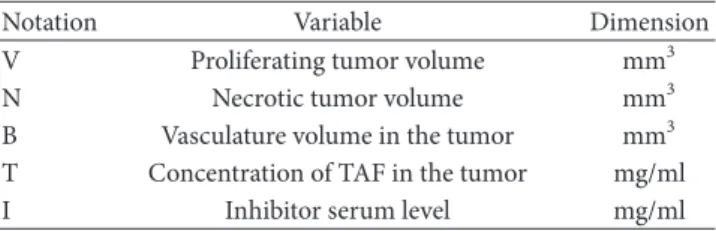
Table 1: State variables of the model.
Notation Variable Dimension
V Proliferating tumor volume mm3
N Necrotic tumor volume mm3
B Vasculature volume in the tumor mm3
T Concentration of TAF in the tumor mg/ml
I Inhibitor serum level mg/ml
density, when all tumor cells are sufficiently supported; in other words,𝑟V= 1. In accordance with biological results [43–
45], we assume that the vasculature is present in the living part of the tumor; thus the vasculature density is interpreted as density of blood vessels in the living (nonnecrotic) part of the tumor and is calculated as[𝐵] = 𝐵/𝑉. Regarding the validity range of the model, we assume that the inequality [𝐵] < [𝐵]𝑖𝑑holds at all times (in other words, we assume that the tumor is never fully vascularized).
The supported ratio of the tumor (𝛾) is computed as 𝛾 = (1 − 𝑟V) 𝑓𝑃(𝑉𝑡𝑜𝑡) + 𝑟V (7) which may be viewed as a linear homotopy in 𝑟V ∈ [0, 1]
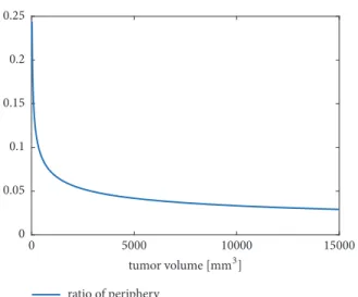
between the constant 1 function and the function𝑓𝑃(𝑉𝑡𝑜𝑡), which is also between zero and one. Thus𝛾 ∈ [0, 1]also holds. The interpretation is that𝑓𝑃(𝑉𝑡𝑜𝑡)denotes a function that describes the ratio of tumor cells on the periphery of the tumor, which receive nutrients from outside of the tumor, so they are well supported. Naturally, this ratio depends on the actual total tumor volume𝑉𝑡𝑜𝑡. More precisely, in our terms, the periphery of the tumor is the outer shell of the sphere of our model, composed by tumor cells, which are closer to the surface of the tumor than the diffusion distance.
According to [33], we assume the diffusion distance to be 150 𝜇𝑚. The ratio of periphery cells depends upon the radius of the tumor, which can be expressed from the tumor volume 𝑉, according to the following simple derivation. Based on the tumor volume, we may derive the tumor radius (in mm) as
𝑉𝑡𝑜𝑡= 4 3𝜋𝑟3 𝑟 =√ 3𝑉3 𝑡𝑜𝑡
4𝜋 .
(8)
If𝑟 ≤ 0.15, there is no tumor core. Assuming𝑟 > 0.15, the volume of the tumor core is
𝑉𝐶=4
3𝜋 (𝑟 − 0.15)3, (9) And thus the volume of the periphery is
𝑉𝑃= 𝑉𝑡𝑜𝑡− 𝑉𝐶, (10) and finally the function𝑓𝑃(𝑉𝑡𝑜𝑡)is derived as
𝑓𝑃(𝑉𝑡𝑜𝑡) = 𝑉𝑃
𝑉𝑡𝑜𝑡. (11)
0 0.05 0.1 0.15 0.2 0.25
ratio of periphery
tumor volume [GG3]
0 5000 10000 15000
Figure 1: The function𝑓𝑃(𝑉𝑡𝑜𝑡)describing the ratio of periphery cells in the range of 20-15000 mm3tumor volume.
If the tumor radius is below the diffusion distance, all cells are considered as periphery cells. The function 𝑓𝑃(𝑉𝑡𝑜𝑡) describing the ratio of periphery cells in the range of 20- 15000 mm3 is depicted in Figure 1 (according to [8], in the time of the first measurement, the volume of the tumors is about 50-60 mm3).
Now let us return our focus to the auxiliary variable𝛾.
The consideration behind the form of function (7) is that we assume two possible ways by which a tumor cell may get nutrient support. On one hand, if it is at the periphery of the tumor, it gets nutrients from the environment of the tumor via diffusion. On the other hand, if it is inside the tumor near a blood vessel, it also receives nutrient supply. The properties of function (7) reflect these considerations. We may see that if the tumor is composed only (or because of the approximation mostly) periphery cells or is almost fully vascularized (𝑟V ≃ 1), the value of𝛾 is approximately 1. In addition, at a fixed value of𝑟V, it increases as the value of𝑓𝑃(𝑉𝑡𝑜𝑡)is increased, and at a fixed vale of𝑓𝑃(𝑉𝑡𝑜𝑡), the value of𝛾is increased as𝑟V increases (to put it simple, it is monotonically increasing in both variables).
Now, as we have discussed the interpretation of the auxiliary variables and the corresponding assumptions, we may return to the state equations. Equation (1) describes the tumor growth. The formula originates from the assumption that the well-supported part of the tumor volume (𝛾𝑉) proliferates at the rate𝑐𝑔, while the unsupported volume𝑉𝑢 necrotizes at the rate𝑐𝑛.
Equation (3) formalizes the dynamics of the vasculature, which may increase by two ways. On one hand, the term 𝑐𝑒V ̇𝑉𝑡𝑜𝑡describes the internalization of new vasculature from the environment as the tumor grows, and on the other hand the term𝑐V𝑇𝐵describes the formation of new blood vessels from existing ones in response to the TAF.
Equation (2) corresponds to necrotic volume. The impor- tance of formally describing the process of necrosis lies in the fact that necrotized cells neither proliferate nor contribute
to TAF production, so they must be distinguished from the general tumor volume.
Equations (4) and (5) describe the dynamics of TAF and the inhibitor concentration, respectively. The terms
𝑐𝑇𝑉𝑢
𝑉 − 𝑞𝑇𝑇 (12)
of (4) describe that the production of TAF is proportional to the ratio of unsupported cells𝑉𝑢/𝑉and takes place at rate 𝑐𝑇, while it is cleared at the rate𝑞𝑇from the tumor. In the case of the inhibitor, the source is the injection (the input)𝑢, while based on [28], we assume that its clearance takes place according to Michaelis-Menten kinetics. The terms
𝑐ℎ 𝑇𝐼
𝐸𝐷50+ 𝐼 (13)
and
𝑘𝑉𝑐ℎ 𝑇𝐼
𝐸𝐷50+ 𝐼 (14)
in (4) and (5), respectively, correspond to the reaction in which the inhibitor binds the TAF molecule. Also, based on [28], the dynamics of the inhibition are considered assuming Michaelis-Menten kinetics with Michaelis-Menten constant 𝐸𝐷50(effective median dose).
The variable 𝑘𝑉 corresponds to the consideration that the concentrations of TAF (𝑇) and the inhibitor (𝐼) are not interpreted in the same volume (the compartment in the former case is the tumor; the volume in the latter case is the plasma).𝑘𝑉is the ratio of these volumes and can be computed as
𝑘𝑉= 𝑉𝑡𝑜𝑡
1460 (15)
where the value 1460 stands for the average blood volume of a mice in𝜇𝑚3, in which the concentration of the inhibitor is interpreted [46].
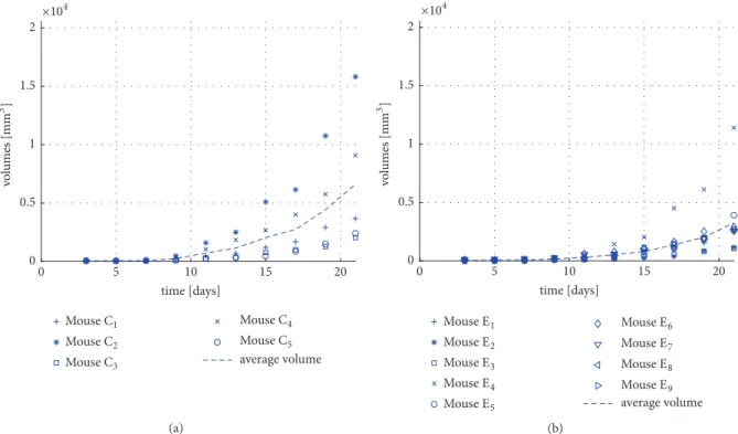
2.2. Model Parameters. Some parameters of the model were taken from the literature (see Table 2), while the remaining parameters were estimated using experimental data originat- ing from mice. S´api et al. [8] carried out experiments, where C57Bl/6 mice with C38 colon adenocarcinoma were treated with bevacizumab using two different therapies.
(i) Therapy 1 (protocol-based treatment): five mice (mice C1-C5) were injected with 0.171 mg/ml bevacizumab at day 3 of the treatment (day 0 is considered as the day of the tumor implantation) (see Figure 2(a)).
(ii) Therapy 2 (daily, quasi-continuous small amount administration): nine mice (mice E1-E9) received9.5⋅
10−4mg/ml injection of bevacizumab each day for 18 days from day 3 (see Figure 2(b)).
The nominal parameter set of the model was determined using the average of measurements as reference and mini- mizing the mean square error of the deviance between the
average volume
×104
Mouse#1 Mouse#2 Mouse#3
Mouse#4
Mouse#5 5
0 10 15 20
time [days]
0 0.5 1 1.5 2
volumes [GG3 ]
(a)
average volume
×104
Mouse%1 Mouse%2
Mouse%3 Mouse%4
Mouse%5
Mouse%6
Mouse%7
Mouse%8 Mouse%9 5
0 10 15 20
time [days]
0 0.5 1 1.5 2
volumes [GG3]
(b)
Figure 2: (a) The measured tumor volumes for mice C1-C5 that received therapy 1 and their average. (b) The measured tumor volumes for mice E1-E9 that received therapy 2 and their average.
simulated and measured total volumes using the combination of particle swarm global optimization method [47] and the
“nlinfit” function of MATLAB. During the simulations, the initial volume of the tumor was assumed to be equal to 5 mm3, while the initial values of all other state variables were assumed to be 0. To capture the qualitatively different response of tumor growth to the two different protocols, both average curves (corresponding to protocols 1 and 2) were used simultaneously for the purpose of parameter estimation.
While initial guess of the parameters was determined by the particle swarm global search method, the final values of the parameters were obtained using the “nlinfit” function. From the results of this function, the 95% confidence intervals (CI95) were determined using the function “nlparci.”
In order to potentially achieve a global optimum with the resulting parameter set, the estimation procedure was started from several initial coordinates in the parameter space. Dur- ing parameter estimation, the average measurement results of both protocols were used to capture the qualitatively different response of the system to different inputs. Table 2 summarizes the model parameters. These parameters are to be referenced as nominal parameters in the further discussion and are denoted as𝜃𝑛𝑜𝑚.
In addition, to quantify parameter variance in the context of single trajectories, the model was fitted also for single growth curves as described in the Appendix.
Most estimated parameters of the model are hard to mea- sure individually (in fact some of them are only interpreted inside the framework of this model) and no data are available on them which could serve as basis for comparison.
3. Results and Discussion
3.1. Fitting the Model to Measurement Data. In this subsec- tion, we compare the model behavior and parameter values to measurement data. Figure 3 shows the fit of the model simulation output (total volume) to the experimental data sets that were used for the parameter estimation (therapy 1 and therapy 2). As it can be seen in the figures, the model sufficiently reproduces the measured growth trajectories, and the better fit is achieved in the case of therapy 2. For the sake of clarity, we note that since the average curve of measurement results was used for parameter estimation, the number of mice used in the experiments did not influence the objective function (in other words, this is not the reason for better fit in the case of therapy 2). To quantify the fit, we introduce the normalized squared deviation (NSD) as
𝑁𝑆𝐷 = ∑𝑡𝑆(𝑉𝑡𝑜𝑡(𝑡𝑆) − 𝑉𝑡𝑜𝑡𝑀(𝑡𝑆))2
𝑡𝑠 (16) where 𝑉𝑡𝑜𝑡 is the simulated total volume (𝑉𝑡𝑜𝑡 = 𝑉 + 𝑁) and𝑉𝑡𝑜𝑡𝑀is the measured total volume.𝑡𝑆 stands for the set of sample times, corresponding to days 3, 5, 7, 9, 11, 13, 15, 17, 19, and 21 in this case, while |𝑡𝑆| denotes the number of sample days. Normalization by the number of days is required, because we will use this measure later as well in the case of experimental data, where the number of sample points is lower. According to this measure, the representative values are𝑁𝑆𝐷𝑇1= 5.5614 ⋅ 105and𝑁𝑆𝐷𝑇2= 6.0609 ⋅ 104𝑚𝑚6in the case of therapy 1 and therapy 2, respectively.
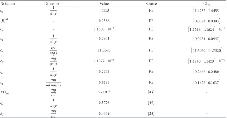
Table 2: Nominal model parameters (𝜃𝑛𝑜𝑚) and their dimension, source, and 95% confidence interval (CI95). PE stands for parameter estimation.
Notation Dimension Value Source CI95
𝑐𝑔 1
𝑑𝑎𝑦 1.4353 PE [1.4252 1.4455]
[𝐵]𝑖𝑑 - 0.0388 PE [0.0383 0.0393]
𝑐𝑒V - 1.1586 ⋅ 10−3 PE [1.1548 1.1624] ⋅ 10−3
𝑐𝑛 1
𝑑𝑎𝑦 0.0941 PE [0.0934 0.0947]
𝑐V 𝑚𝑙
𝑚𝑔 𝑠 11.6690 PE [11.6060 11.7320]
𝑐𝑇 𝑚𝑔
𝑚𝑙 𝑠 1.1377 ⋅ 10−2 PE [1.1330 1.1423] ⋅ 10−2
𝑞𝑇 1
𝑑𝑎𝑦 0.2473 PE [0.2466 0.2480]
𝑐ℎ 𝑚𝑔
𝑚𝑙 𝑚𝑚3𝑠 0.1633 PE [0.1628 0.1637]
𝐸𝐷50 𝑚𝑔
𝑚𝑙 5 ⋅ 10−5 [48] -
𝑞𝐼 1
𝑑𝑎𝑦 0.5776 [49] -
𝑘𝐼 𝑚𝑔
𝑚𝑙 0.4409 [28] -
average measured volume
×104
Mouse#1 Mouse#2
Mouse#3
Mouse#4 Mouse#5 simulated6NIN
5 10 15 20
0
time [days]
0 0.5 1 1.5 2
volumes [GG3 ]
(a)
average volume Mouse%1
Mouse%2
Mouse%3 Mouse%4 Mouse%5
Mouse%6
Mouse%7 Mouse%8 Mouse%9
simulated6NIN
5 10 15 20
0
time [days]
0 2000 4000 6000 8000 10000 12000 14000
volumes [GG3]
(b)
Figure 3: Measured and simulated tumor volumes in the case of therapy 1 (a) and therapy 2 (b).
The possible reason for the better fit in the case of the quasi-continuous therapy may be that the average of the measurements provides a more smooth, exponential- like curve in this case, which was possibly more easy to be achieved by the model.
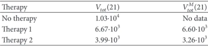
The final volume of the tumor according to simulation results is 6670 mm3in the case of therapy 1 and 3993 mm3in the case of therapy 2. Considering the data described in Sec- tion 2.2, the final average measured volumes (corresponding to day 21) were 6604 and 3257 mm3in the cases of therapy 1 and therapy 2, respectively.
3.2. Model Validation
3.2.1. Qualitative Validation. In this subsection, we analyze and compare the dynamic behavior of key model variables in the cases of no therapy, therapy 1, and therapy 2 defined in Section 2.2.
Figure 4 depicts the trajectory of𝛾and𝑟Vin the various cases.
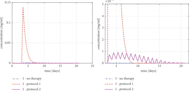
In general, it can be said that, in the beginning, when the tumor is small, due to the high ratio of periphery cells,𝛾(i.e., the ratio of the well-supported tumor cells) is high. However, as the tumor grows, the ratio of peripherial cells and so𝛾also decrease. The trajectories of the various cases differ only after day 6. The reason for this is that the process of angiogenesis becomes significant only if a large part of unsupported cells and TAF is already present, and the inhibition of the process becomes important only in this period. This is also shown in Figure 4(b), where it can be seen that the various cases regarding the vascularization ratio (𝑟V) differ only after day 6. Furthermore, it can be seen in Figure 4 that both𝛾 and 𝑟V remain in the range[0, 1]as assumed during the model formulation. Figure 5 depicts the inhibitor concentration in the cases of therapy 1 and therapy 2 (in the case of no therapy, the inhibitor concentration is constant zero during the simulation). It can be seen in the figure that, in the case of therapy 1, the concentration is several orders of magnitude higher compared to therapy 2.
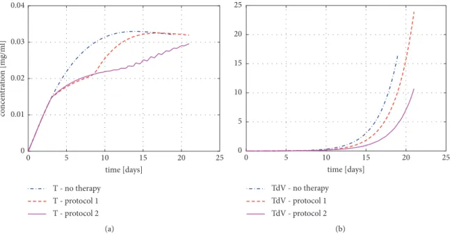
Figure 6 depicts the concentration of TAF (𝑇) and the term𝑐V𝑇𝐵of (3) (corresponding ot TAF-dependent vascular- ization) in response to the various levels of the inhibitor in the case of different therapies.
In this figure (Figure 6(a)), it can be seen that the concentration of TAF (𝑇) around days 3-8 is almost the same in the case of therapy 1 and therapy 2, although the concentration of the inhibitor (𝐼) differs on the orders of magnitude. The explanation for this is the effective median dose (𝐸𝐷50) of the inhibitor, which defines the inhibitor level at which the effect of the drug saturates. We have to note that this parameter was not subject to estimation but it was taken from the article [48]. Figure 6(b) depicts that from the time when the large bolus has been cleared in the case of therapy 1 (around day 13), the TAF-dependent vascularization (TdV) becomes significantly different in the case of the two therapies.
Since the volume trajectories of the model follow an exponential-like fashion in all cases, they are maybe not so
Table 3: Simulated and measured average total volumes on day 21 (mm3).
Therapy 𝑉𝑡𝑜𝑡(21) 𝑉𝑡𝑜𝑡𝑀(21)
No therapy 1.03⋅104 No data
Therapy 1 6.67⋅103 6.60⋅103
Therapy 2 3.99⋅103 3.26⋅103
Table 4: Simulated and measured average total volumes on day 19 (mm3).
Therapy 𝑉𝑡𝑜𝑡(19) 𝑉𝑡𝑜𝑡𝑀(19)
No therapy 4.68⋅103 6.15⋅103
Therapy 1 3.10⋅103 4.44⋅103
Therapy 2 2.13⋅103 2.03⋅103
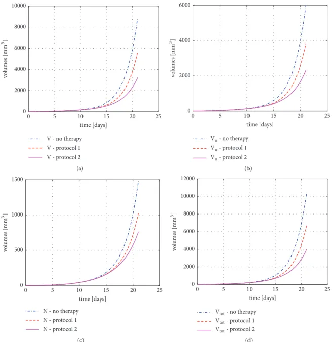
informative as, for example, the plot of𝛾, but for the sake of completeness, they are depicted in Figure 7.
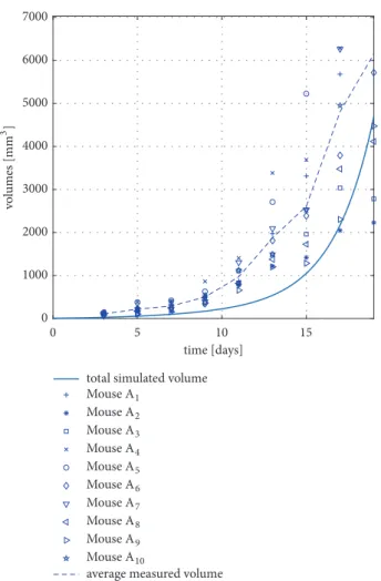
3.2.2. Validation against Measurement Data with No Therapy.
In phase I of the experiments described in [8], the experimen- tal animals received no treatment. In this case, the length of the experiment was only 19 days (compared to 21 days in all other experiments discussed before and depicted in Figure 2).
The measurement data originating from this experiment was used to validate the model. Figure 8 shows the results of the model validation.
The measure of the fit introduced in (16) gives a value of 𝑁𝑆𝐷𝑁𝑇 = 1.5451 ⋅ 106mm6 in this case (the lower index corresponds to “no therapy”). If one compares this value to the NSD values corresponding to the experimental data to which the model was fitted (see Section 3.1), or examines the figures, it can be seen that the error of the fit is one order of magnitude higher in this case (since the no-therapy case was not considered during parameter estimation). On the other hand, taking into account the significant variation among experimental animals as well, the the model output in the case of no therapy provides an acceptable fit with measurement data.
3.2.3. Validation regarding Final Tumor Volume Values in Various Cases. As in control applications, for which the current model is primary proposed, the usual aim is to minimize the final volume of the tumor (under, e.g., con- straints corresponding to the total applied drug quantity); it is important to compare the final tumor sizes. As the final day of the experiments was different in the no-therapy case and therapies 1 and 2, Tables 3 and 4 summarize the simulated and measured tumor volumes on days 19 and 21.
For the sake of comparison to previous literature results, let us note that the simulated volume on day 19 assuming no therapy is1.85 ⋅ 104 in the case of the model described in [28] (this value has been obtained by the reproduction of the model described in [28]). Comparing the differences of the values, we may say that the validity of the proposed model compared to [28] is significantly better regarding the final volume in the no-therapy case.
0.2 0.3 0.4 0.5 0.6
- no therapy
- protocol 1
- protocol 2
5 10 15 20 25
0
time [days]
(a)
0 0.1 0.2 0.3
LP- no therapy LP- protocol 1 LP- protocol 2
5 10 15 20 25
0
time [days]
(b)
Figure 4: (a) Ratio of the well-supported tumor cells (𝛾) in the case of various therapies; (b) vascularization ratio (𝑟V) in the case of various therapies.
I - no therapy I - protocol 1 I - protocol 2
I - no therapy I - protocol 1 I - protocol 2
×10−3
0 0.05 0.1 0.15
concentration [mg/ml]
5
0 10 15 20 25
time [days]
5 10 15 20
time [days]
0 1 2 3 4 5
concentration [mg/ml]
Figure 5: Concentration of the inhibitor (𝐼) in the case of various therapies on two different scales.
3.3. Model Identifiability. In the following two subsections, we present some results related to the parameter sensitivity and structural identifiability of the proposed model.
3.3.1. Parameter Sensitivity of the Model. In this subsection, we analyze the parameter sensitivity of the model for the estimated parameters. The sensitivity analysis is an important tool to characterize how the model parameters affect the simulation output. The presence of very large differences in the sensitivities of parameters may point to identifiability problems.
In order to formalize this analysis, we define the sensitiv- ity measure detailed in the following equation:
𝑆 (̂𝜃) = ∫𝑇
0
(𝑉𝑡𝑜𝑡(𝑡, 𝜃𝑛𝑜𝑚) − ̂𝑉𝑡𝑜𝑡(𝑡, ̂𝜃))2
𝑇 𝑑𝑡 (17)
In (17), 𝜃𝑛𝑜𝑚 denotes the nominal parameter vector detailed in Table 2, while ̂𝜃denotes a perturbed parameter vector. 𝑉𝑡𝑜𝑡(𝜏, 𝜃𝑛𝑜𝑚) and 𝑉̂𝑡𝑜𝑡(𝜏, ̂𝜃) stand for the nominal output (𝑉𝑡𝑜𝑡(𝑡)) of the model and for the output in the case of the perturbed parameter vector, respectively.
T - no therapy T - protocol 1 T - protocol 2
5
0 10 15 20 25
time [days]
0 0.01 0.02 0.03 0.04
concentration [mg/ml]
(a)
0 5 10 15 20 25
TdV - no therapy TdV - protocol 1 TdV - protocol 2
5
0 10 15 20 25
time [days]
(b)
Figure 6: (a) Concentration of TAF (𝑇) in the case of various therapies; (b) TAF-dependent vascularization (TdV) in the case of different therapies.
No-Therapy Case. Table 5 summarizes the results in the no-therapy case. Each row of this table corresponds to a
̂𝜃perturbed parameter vector, in which only one element differs from the nominal𝜃vector (by 20, 10, or 5%).
First, it is conspicuous that the sensitivity to the parameter 𝑐ℎ is zero in this case. The explanation for this is that this parameter corresponds to the effect of the angiogenic inhibitor (𝐼), the concentration of which is constantly 0 in this case. In other words, there is no drug effect in this case, the dynamics of which are affected by this parameter.
Second, we can see in Table 5 that the sensitivity for 𝑐V is equal to the sensitivity of 𝑐𝑇 in the no-therapy case.
The reason for this is that while 𝑐𝑇 corresponds to the synthesis rate of TAF, 𝑐V corresponds to the rate of TAF- dependent vascularization. If no inhibitor is present, there is no difference between an increase in the TAF concentration and a more efficient TAF-driven vascularization (see (3) and (4)). Let us note that if the inhibitor is present, not the whole portion of the synthetized TAF takes part in the blood vessel formation process (since some molecules are binding to the inhibitor); thus the situation is different if input (thus nonzero drug concentration) is also present.
Third, the model is the most sensitive to the parameter𝑐𝑔. This is not surprising, as𝑐𝑔directly affects the dynamics of𝑉 (see (1)) as a proportional term, so its effect in𝑉, which is directly present in the output, is exponential. Apart form𝑐ℎ, 𝑞𝐼, and𝑘𝑉, the model shows the least sensitivity to𝑐𝑛, the rate of necrosis.
Therapy 1. Table 6 shows that the model sensitivity for 𝑐ℎ, the parameter corresponding to the effect of the inhibitor, is relatively low.
Table 7 shows that, in the case of therapy 2, an extreme high sensitivity is experienced in the case of the increase of
parameter𝑐𝑔. Moreover, the sensitivity to𝑞𝐼is also signifi- cantly decreased. As the injections and thus the concentra- tions of the inhibitor (𝐼) are by 2 orders of magnitude lower compared to therapy one (see Figure 5), it is plausible that the exact value of its clearance parameter (𝑞𝐼) has a significantly less effect on the dynamics of the model compared to therapy 1, where a large dose is applied.
Apart from this, the results are similar to the case of therapy 1.
Altogether, based on the results of the sensitivity analysis, it can be said that further experiments focusing solely on pharmacokinetics of the applied drugs are desirable to estimate the parameter 𝑐ℎ decoupled from other model parameters.
3.3.2. Structural Identifiability. Structural identifiability properties of a system describe whether there is a theoretical possibility for the unique determination of system parameters from appropriate input-output measurements or not. It is important to emphasize that identifiability is a property of the model structure. Basic early references for studying identifiability of dynamical systems are [50, 51]. Since the introduction of this concept, multiple approaches have been proposed for the analysis of structural identifiability of various nonlinear system classes, for example, polynomial systems [52] or rational function state-space models [53]. A critical comparison of methods for identifiability analysis is described in [54].
First, let us note that as our model uses the variable[𝐵] = 𝐵/𝑉describing vasculature density, our model falls into the class of rational function state-space models.
Second, let us consider the factors that make the structural identifiability analysis challenging in our case.
Structural identifiability methods usually rely on iterative
V - no therapy V - protocol 1 V - protocol 2 0
2000 4000 6000 8000 10000
volumes [GG3]
5
0 10 15 20 25
time [days]
(a)
6O- no therapy 6O- protocol 1 6O- protocol 2 0
2000 4000 6000
volumes [GG3 ]
5
0 10 15 20 25
time [days]
(b)
N - no therapy N - protocol 1 N - protocol 2 0
500 1000 1500
volumes [GG3]
5
0 10 15 20 25
time [days]
(c)
6NIN- no therapy 6NIN- protocol 1 6NIN- protocol 2 0
2000 4000 6000 8000 10000 12000
volumes [GG3 ]
5
0 10 15 20 25
time [days]
(d)
Figure 7: Volume trajectories of the model (living volume 𝑉, unsupported volume 𝑉𝑢, necrotic volume 𝑁, and total volume 𝑉𝑡𝑜𝑡, corresponding to subfigures (a), (b), (c), and (d), resp.) in the case of various therapies.
Table 5: Sensitivities (𝑆) of the model to the changes of parameters[𝐵]𝑖𝑑,𝑐𝑔,𝑐𝑒V,𝑐𝑛,𝑐V,𝑐𝑇,𝑞𝑇,𝑐ℎ,𝑞𝐼, and𝑘𝑉in the no-therapy case. One unit is106mm3.
-20% -10% -5% +5% +10% +20%
[𝐵]𝑖𝑑 0.1321 0.0240 0.0052 0.0040 0.0143 0.0462
𝑐𝑔 0.4715 0.1601 0.0467 0.0640 0.2996 1.6456
𝑐𝑒V 0.0653 0.0173 0.0044 0.0047 0.0193 0.0821
𝑐𝑛 0.0072 0.0017 0.0004 0.0004 0.0016 0.0061
𝑐V 0.2287 0.0769 0.0224 0.0309 0.1454 0.8147
𝑐𝑇 0.2287 0.0769 0.0224 0.0309 0.1454 0.8148
𝑞𝑇 0.5561 0.0868 0.0176 0.0120 0.0405 0.1185
𝑐ℎ 0 0 0 0 0 0
Table 6: Sensitivities (𝑆) of the model to the changes of parameters[𝐵]𝑖𝑑,𝑐𝑔,𝑐𝑒V,𝑐𝑛,𝑐V,𝑐𝑇,𝑞𝑇,𝑐ℎ,𝑞𝐼, and𝑘𝑉in the case of therapy 1. One unit is106mm3.
-20% -10% -5% +5% +10% +20%
[𝐵]𝑖𝑑 0.2926 0.0525 0.0114 0.0086 0.0305 0.0975
𝑐𝑔 0.9383 0.3259 0.0962 0.1353 0.6422 3.6265
𝑐𝑒V 0.1375 0.0368 0.0095 0.0102 0.0420 0.1807
𝑐𝑛 0.0181 0.0043 0.0011 0.0010 0.0039 0.0149
𝑐V 0.4498 0.1518 0.0442 0.0611 0.2889 1.6242
𝑐𝑇 0.4594 0.1559 0.0456 0.0634 0.3011 1.7086
𝑞𝑇 0.9364 0.1493 0.0305 0.0213 0.0720 0.2128
𝑐ℎ 0.0100 0.0023 0.0005 0.0005 0.0019 0.0069
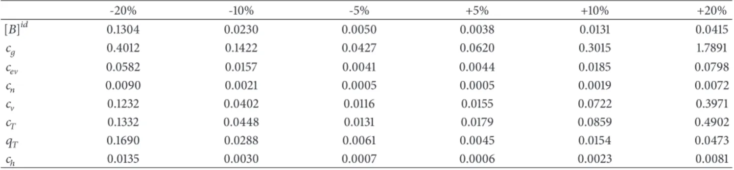
Table 7: Sensitivities (𝑆) of the model to the changes of parameters[𝐵]𝑖𝑑,𝑐𝑔,𝑐𝑒V,𝑐𝑛,𝑐V,𝑐𝑇,𝑞𝑇,𝑐ℎ,𝑞𝐼, and𝑘𝑉in the case of therapy 2. One unit is107mm3.
-20% -10% -5% +5% +10% +20%
[𝐵]𝑖𝑑 0.1304 0.0230 0.0050 0.0038 0.0131 0.0415
𝑐𝑔 0.4012 0.1422 0.0427 0.0620 0.3015 1.7891
𝑐𝑒V 0.0582 0.0157 0.0041 0.0044 0.0185 0.0798
𝑐𝑛 0.0090 0.0021 0.0005 0.0005 0.0019 0.0072
𝑐V 0.1232 0.0402 0.0116 0.0155 0.0722 0.3971
𝑐𝑇 0.1332 0.0448 0.0131 0.0179 0.0859 0.4902
𝑞𝑇 0.1690 0.0288 0.0061 0.0045 0.0154 0.0473
𝑐ℎ 0.0135 0.0030 0.0007 0.0006 0.0023 0.0081
computation of (Lie-) derivatives of the output (see, e.g., [55], on which the software used later is based).
For identifiability analysis, let us consider a reduced version of the proposed model, which assumes no input (no antiangiogenic drug is present). The simplified form of the model is described by (18)-(21). As we will see, this submodel already poses a challenge regarding identifiability due to the complexity of the resulting equations.
𝑑𝑉
𝑑𝑡 = 𝑐𝑔𝛾𝑉 − 𝑐𝑛(1 − 𝛾) 𝑉 (18) 𝑑𝑁
𝑑𝑡 = 𝑐𝑛(1 − 𝛾) 𝑉 (19)
𝑑𝐵
𝑑𝑡 = 𝑐𝑒V𝑐𝑔𝛾𝑉 + 𝑐V𝑇𝐵 (20) 𝑑𝑇
𝑑𝑡 = 𝑐𝑇(1 − 𝛾) − 𝑞𝑇𝑇 (21) In this case, if only the total volume may be measured (as in the case of our measurements used for the parameter estimation),
𝑦 = 𝑉𝑡𝑜𝑡= 𝑉 + 𝑁
̇𝑦 = ̇𝑉 + ̇𝑁 = 𝑐𝑔𝛾𝑉 (22) If we consider further derivatives,
̈𝑦 = 𝑐𝑔( ̇𝛾𝑉 + ̇𝑉𝛾) (23)
where
𝛾 = (1 − 𝑟V) 𝑓𝑃(𝑉𝑡𝑜𝑡) + 𝑟V= (1 − 𝑟V) 𝑓𝑃(𝑉𝑡𝑜𝑡) + 𝑟V (24) ([𝐵]𝑖𝑑− [𝐵]
[𝐵]𝑖𝑑 ) 𝑓𝑃(𝑉𝑡𝑜𝑡) + (1 − [𝐵]𝑖𝑑− [𝐵]
[𝐵]𝑖𝑑 ) (25) It is easy to se that, in ̇𝛾, on one hand, the derivative of the function𝑓𝑃(𝑉𝑡𝑜𝑡)appears, and, on the other hand, the derivative of [𝐵] = 𝐵/𝑉 is also present. These are long and complicated expressions, the higher-order derivatives of which are needed in the further steps.
Based on the above considerations, for the structural identifiability analysis, we use the freely available GenSSI [56, 57] software, which is able to handle complex expressions with the help of computer-algebra methods. GenSSI imple- ments iteratively the generating series method, as presented in [58], with the help of identifiability tableaus, as described in [55].
According to the results of this software, the parameter𝑐𝑔 of the model is structurally globally identifiable, but neither positive (structural global/local identifiability) nor negative (structural nonidentifiability) results are obtained for other parameters. This result is based on 7𝑡ℎ-order Lie-derivatives, which has been proven to be the computational limit in our case.
Nevertheless, let us discuss this topic a bit further from the point of view of possible future measurements with regard to the proposed model. In the recent years, multiple imaging techniques have been developed, which
time [days]
0 1000 2000 3000 4000 5000 6000 7000
total simulated volume
average measured volume Mouse A1
Mouse A10 Mouse A2 Mouse A3 Mouse A4 Mouse A5 Mouse A6 Mouse A7 Mouse A8 Mouse A9
5 10 15
0 volumes [GG3]
Figure 8: Measured and simulated tumor volumes in the case of no therapy.
allow the 3D reconstruction of vascular microstructures:
Doppler optical frequency domain imaging [29] and func- tional photoacoustic microscopy [30] are used today already in in vivo setups to map vascular networks, while dif- fusible iodine-based contrast-enhanced computed tomog- raphy [31] may be used in terminal experimental ani- mals.
If these methods will be applicable in the case of animals used in the experiments, total tumor volume 𝑉𝑡𝑜𝑡 will be accessible during measurements together with the total vasculature volume 𝐵. Interpreted for our case, this will mean that we will have two observables 𝑦1 = 𝑉𝑡𝑜𝑡 and 𝑦2 = 𝐵. If we rerun the structural identifiability analysis with this new model output, we get the result that 𝑐𝑔, 𝑐𝑒V, [𝐵]𝑖𝑑, and 𝑐𝑛 are structurally globally identifiable (and no result is obtained for other parameters, similar to the previous case, so they might be or might be not identifiable). In this case, the maximum order of the Lie- derivatives, for which the computation was feasible, was the 6𝑡ℎorder.
The complete identifiability tableaus of the reduced model are depicted in Figure 9. For the interpretation of these tableaus, see [55] or the GenSSI UserGuide [56].
Based on the above, it may be suspected that the model will have beneficial properties shall it be fitted for measure- ments planned to be carried out in the foreseeable future.
3.4. Extension of the Model in order to Account for Combined Therapy. In the clinical practice, antiangiogenic drugs are often used together with conventional cytotoxic substances.
In this setup, while the cytotoxic agent enhances the degen- eration/necrosis of tumor cells, the antiangiogenic drugs are resposible for cutting the tumor from metabolic support via the inhibition of angiogenesis. Several results have been pub- lished recently corresponding to these combined therapies [59, 60].
Models with predictive power regarding the efficiency of combined therapies and model-based optimization of such treatments are not prevalent in literature. Some initial results on the optimization of combined therapies are described in [61], using the model of [35].
As the proposed model is taking into account vasculature and tumor cell dynamics in a differentiated way, it is able to distinguish between qualitatively different inputs related to different therapeutic agents. As a consequence, the proposed model may be easily extended to consider not only angiogenic drugs but also cytotoxic drugs. Let us consider the following modified state-space model described in the following equa- tions:
𝑑𝑉
𝑑𝑡 = 𝑐𝑔𝛾𝑉 − 𝑐𝑛𝑉𝑢− 𝑐𝑐𝐶𝑉
𝐾𝐶+ 𝑉 (26)
𝑑𝑁
𝑑𝑡 = 𝑐𝑛𝑉𝑢+ 𝑐𝑐𝐶𝑉
𝐾𝐶+ 𝑉 (27)
𝑑𝐵
𝑑𝑡 = 𝑐𝑒V ̇𝑉𝑡𝑜𝑡+ 𝑐V𝑇𝐵 (28) 𝑑𝑇
𝑑𝑡 = 𝑐𝑇𝑉𝑢
𝑉 − 𝑞𝑇𝑇 − 𝑐ℎ 𝑇𝐼
𝐸𝐷50+ 𝐼 (29) 𝑑𝐼
𝑑𝑡 = 𝑢1− 𝑞𝐼 𝐼
𝑘𝐼+ 𝐼 − 𝑘𝑉𝑐ℎ 𝑇𝐼
𝐸𝐷50+ 𝐼 (30) 𝑑𝐶
𝑑𝑡 = 𝑢2− 𝑞𝐶𝐶 (31)
First, the new equation (31) describes the time evolution of the cytotoxic drug, the injection of which is described by the term 𝑢2. To clarify notations, the injection of the angiogenic inhibitor is denoted by 𝑢1 in this case. The term𝑞𝐶𝐶describes the clearance of the cytotoxic drug; the parameter 𝑞𝐶 denotes its clearance rate. In this case, we assume a simple clearance (no saturation dynamics). The reason for this is on one hand that this approach requires less parameters, and on the other hand as long as the exact identity of the cytotoxic drug is unknown, the dynamical features of its clearance can not be precisely determined (of course the clearance dynamics may be later refined).
The effect of the cytotoxic drug is modeled in this case as an enzymatic reaction, in which the cytotoxic drug acts as an
1 2 3 4 5 6 7 8
Identifiability tableau
["]C> #A #?P #H #P #4 K4 (a)
Identifiability tableau
2 4 6 8 10 12 14
["]C> #A #?P #H #P #4 K4 (b)
Figure 9: Complete identifiability tableaus of the reduced model in the case when the output is𝑉𝑡𝑜𝑡(a) and in the case when the output is [𝑉𝑡𝑜𝑡, 𝐵](b).
enzyme, turning living cells to necrotic cells. This mechanism is described by the term
− 𝑐𝑐𝐶𝑉
𝐾𝐶+ 𝑉 (32)
in (26) and by the complementary term 𝑐𝑐𝐶𝑉
𝐾𝐶+ 𝑉 (33)
in (27). 𝑐𝑐 and 𝐾𝐶 are new parameters describing the effi- ciency of the cytotoxic drug in enzymatic context assuming Michaelis-Menten kinetics.
This way the effects of the two drugs are considered in qualitatively different ways in the model. While the antian- giogenic drug acts explicitly on the formation of new blood vessels by binding to TAF and thus inhibiting angiogenesis, the cytotoxic drug acts as an enzyme, driving living tumor cells to necrosis, independent of the actual vascular state of the tumor.
4. Conclusions and Future Work
In this article, we formulated a dynamic model of vascular tumor growth, which accounts for the vasculature and TAF concentration development of the tumor and thus is able to reproduce the phenomenon of the angiogenic switch.
We validated the model against volume measurement data originating from experiments on mice and found that the model provides a good fit for tumor volume data in both cases of the two analyzed therapies. The extension of the model described in Section 3.4 makes the model capable of accounting for qualitatively different effect of antiangiogenic and cytotoxic drugs.
When comparing the proposed model to literature results, we may state the following. Regarding the model in
[28] (considering the extended model described therein), the proposed approach uses more state variables (5 vs 3) and holds more parameters (12 versus 8) but describes vasculature dynamics as well. This feature will allow us to fit the model to dynamical vasculature data, hopefully available in the foreseeable future, and thus get a more precise dynamical representation of angiogenesis-dependent tumor growth and its inhibition. Furthermore, the validity of the proposed model compared to [28] seems better regarding the no- therapy case.
Comparing the model described in the current article to [35], we see that although the model described in [35]
accounts for vasculature dynamics as well, it uses more state variables (7 versus 5) and significantly more parameters (22 versus 12). Furthermore, the model in [35] was fitted only for measurement data originating from protocol 1, while the proposed model has been validated against both protocol 1 and protocol 2. Similar to the model described in [35], the model proposed in the current article also allows for the analysis of combined therapies, as done in the article in [61].
Regarding future work, in the framework of the project Tamed Cancer (ERC grant agreement number 679681), animal experiments (mice) aiming to characterize the vas- culature development during tumor growth are planned in the near future. These experiments will provide reference data for both vasculature volumes and tumor volumes, so we will be able to fit the model in either dimension against experimental data. This will allow further validation, refinement, or recalibration of the model.
Experiments regarding the efficiency of various com- bined therapies are also expected in the future, which will serve as reference scenarios regarding the identification of the extended model described in Section 3.4.
Once the model is identified and validated from multiple aspects, studies on therapy optimization in open-loop and closed-loop setup will take place.
measured volume simulated volume -;EN
simulated volume -HIG
protocol 1, mouse C
0 1000 2000 3000 4000 5000 6000
volumes [GG3 ]
5
0 10 15 20 25
time [days]
(a)
measured volume simulated volume -;EN
simulated volume -HIG
protocol 1, mouse C
0 2000 4000 6000 8000 10000
volumes [GG3]
5
0 10 15 20 25
time [days]
(b)
measured volume simulated volume -;EN simulated volume -HIG
protocol 1, mouse C
0 1000 2000 3000 4000 5000 6000
volumes [GG3]
5
0 10 15 20 25
time [days]
(c)
time [days]
×104
0 5 10 15 20 25
measured volume simulated volume -;EN simulated volume -HIG
protocol 1, mouse C
0 0.5 1 1.5 2
volumes [GG3 ]
(d)
time [days]
0 1000 2000 3000 4000 5000 6000
volumes [GG3 ]
0 5 10 15 20 25
measured volume simulated volume -;EN
simulated volume -HIG
protocol 1, mouse C
(e)
Figure 10: Fitting the model to individual trajectories in the case of therapy 1: simulated output (with the parameters obtained from fitting the model to the specific trajectory (𝜃𝑎𝑘𝑡), simulated output with nominal parameters (𝜃𝑛𝑜𝑚), and measured output.)