for Brain Tumour Segmentation from Multispectral MR Image Data

for Brain Tumour Segmentation from Multispectral MR Image Data

Agnes Gy˝´ orfi^1,2, Zolt´an Karetka-Mezei¹, David Icl˘anzan¹, Levente Kov´acs², and L´aszl´o Szil´agyi^1,2(B⁾

1 Computational Intelligence Research Group,

Sapientia - Hungarian University of Transylvania, Tˆırgu Mure¸s, Romania {gyorfiagnes,iclanzan,lalo}@ms.sapientia.ro, karetkaz@yahoo.com

2 University Research, Innovation and Service Center (EKIK), Obuda University, Budapest, Hungary´

{kovacs.levente,szilagyi.laszlo}@nik.uni-obuda.hu

Abstract. Absolute values in magnetic resonance image data do not say anything about the investigated tissues. All these numerical values are relative, they depend on the imaging device and they may vary from session to session. Consequently, there is a need for histogram normaliza- tion before any other processing is performed on MRI data. The Brain Tumor Segmentation (BraTS) challenge organized yearly since 2012 con- tributed to the intensification of the focus on tumor segmentation tech- niques based on multi-spectral MRI data. A large subset of methods developed within the bounds of this challenge declared that they rely on a classical histogram normalization method proposed by Ny´ul et al. in 2000, which supposed that the corrected histogram of a certain organ composed of normal tissues only should be similar in all patients. How- ever, this classical method did not count with possible lesions that can vary a lot in size, position, and shape. This paper proposes to perform a comparison of three sets of histogram normalization methods deployed in a brain tumor segmentation framework, and formulates recommenda- tions regarding this preprocessing step.

Keywords: Magnetic resonance imaging

·

·

Tumor segmentation

·

1 Introduction

The ever growing number of medical imaging devices cannot be followed by the number of human experts who are able to reliably evaluate the image records.

This project was supported by the Sapientia Foundation – Institute for Scientific Research. The work of L. Kov´acs was supported by the European Research Council (ERC) under the European Union’s Horizon 2020 research and innovation programme (grant agreement No 679681). The work of L. Szil´agyi was supported by the Hungarian Academy of Sciences through the J´anos Bolyai Fellowship program.

c Springer Nature Switzerland AG 2019

I. Nystr¨om et al. (Eds.): CIARP 2019, LNCS 11896, pp. 375–384, 2019.

https://doi.org/10.1007/978-3-030-33904-3_35

This is causing an intensifying need for automated algorithms that can filter out the surely negative cases and recommend the suspected positives to be inves- tigated by the human experts. The most important requirement for such auto- mated algorithms is to minimize the number of false negatives, which means that they have to be sensitive to any sort of lesions in the tissues.

Magnetic resonance imaging (MRI) is a frequently used technique in the brain tumor detection and segmentation problem, because of its high contrast and relatively good resolution. However, MRI has a serious drawback: the numer- ical values in its records do not directly reflect the imaged tissues. In order to correctly interpret the observed images, it is necessary to adapt them to the context, which is usually performed via histogram normalization. Without this step, comparing two intensity values from two different MRI records would be like comparing the water amount in two bottles by checking only the depth of the water in them and ignoring the shape of the bottles.

Several solutions have been proposed to normalize or standardize the his- tograms of MRI records [1–5]. However, none of them were designed to tackle with focal lesions (tumors, gliomas) that might be present. Some brain tumors grow to 20–30% of the brain volume, which strongly distorts the histogram of any data channel of the MRI histograms. Luckily, normal and tumor tissues look differently in some data channels, and thus we are able to identify the pres- ence of tumors. Normalizing the histograms in batch mode, as it is done by the most popular technique proposed by Ny´ul et al. [1] (referred to as method A1 in the following), and expecting them to look similar whether they contain tumor or not, is prone to damage the segmentation quality. A1 produces a two-step transformation of intensities using some predefined intensity percentiles as land- mark points. Several recent studies report using A1, without giving details of its parametrization [6–16]. Few studies indicate the number of landmark points involved: Soltaninejad et al. [17] mentioned using 12 landmarks, while Pinto et al. [18] seem to be using the S1 setting of the method A1, see details in Sect.3.1. Tustison et al. [19] remarked that a simple linear transformation based method can provide slightly better accuracy than A1, without giving details of their method. Such simple linear transforms were applied in [20–22], without comparing their effect to other histogram normalization methods.

This paper intends to investigate how suitable the above mentioned most popular histogram normalization method is at preprocessing MRI data in a brain tumor segmentation problem. In this order, three sets of algorithms are compared:

1. Method A1, with several settings schemes that affects the number and posi- tion of landmark points;

2. Method A2, which in fact is method A1 with landmark points defined by the fuzzyc-means clustering algorithm [23];

3. Method A3, a simple linear transform, with a single parameter, that gener- alizes the method employed in [20–22].

The rest of the paper is structured as follows: Sect.2 presents the necessary details of background works, Sect.3 gives details of the compared algorithms,

Statistical evaluation

Morphological post−processing

Prediction by ensemble Histogram

normalization

Feature extraction

Ensemble training MRI

data

Dicescores

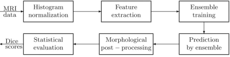
Fig. 1.Block diagram of the evaluation framework.

Sect.4provides a detailed analysis of the obtained results, while Sect.5concludes the study.

2 Background

2.1 Data

This study relies on the 54 low-grade glioma (LGG) volumes of the BraTS 2016 train dataset [24,25]. All MRI records contain four data channels (T1, T2, T1C, FLAIR), each with 155 slices of 240×240 isovolumetric pixels representing one cubic millimeter of brain tissue. Records contain approximately 1.5 mil- lion brain pixels. The ground truth provided by human experts is available for each record, which stands at the basis of training and testing machine learning solution deployed in the segmentation problem.

2.2 Framework

In order to evaluate various histogram normalization techniques, a framework was built that can deploy ensemble learning methods in a tumor segmentation problem based on MRI data. The block diagram of the framework is shown in Fig.1.

In this study we worked with ensembles of binary decision trees (BDT). Each BDT was trained to separate negative and positive pixels based on the feature vectors of 10000 pixels that were randomly selected from the train data set.

During the training process, BDTs were allowed to place nodes at any depth that was necessary. Most BDTs grew to a maximum depth between 20 and 25.

On the other hand, when decision were made by the trained BDTs, the average depth of the leaf making the decision was around depth 8.

The tested histogram normalization methods (see Sect.3) were used as the first step of the data processing, as indicated in Fig.1. The output of each was fed to the further steps, and statistical evaluation results collected for comparison.

2.3 The A1 Method

The histogram normalization method proposed by Ny´ul et al. [1] works as follows:

1. The previously defined target intensity interval is denoted by [α, β].

2. A previously defined set of MRI records R is involved in the process, the number of records is denoted byr. The histogram of each record is extracted.

3. The set of landmark points is defined, for exampleΛ ={plow = 1%, p_L1 = 10%, p_L2 = 20%, . . . , p_L9= 90%, phigh= 99%}. Let us denote the number of inner landmark points byλ(in the previous exampleλ= 9).

4. For all MRI records with index i, i = 1. . . r, the intensity values corre- sponding to the landmark points defined inΛare identified and denoted by y_low⁽ⁱ⁾, y_L1⁽ⁱ⁾, y_L2⁽ⁱ⁾, . . . , y⁽ⁱ⁾_Lλ, y⁽ⁱ⁾_high, respectively.

5. A first transformation step is performed: a linear transformation is designed such a way that mapsy_low⁽ⁱ⁾ to y⁽ⁱ⁾_low=α,y⁽ⁱ⁾_highto y⁽ⁱ⁾_high=β, and applies this linear transform to all intensity values situated between y⁽_lowⁱ⁾ and y_high⁽ⁱ⁾ in the original histogram. The two tails of the histogram is cut, meaning that intensity values belowy_low⁽ⁱ⁾ are transformed toα, and intensity values above y_high⁽ⁱ⁾ are transformed toβ. For any j= 1. . . λ,y⁽ⁱ⁾_Lj is transformed toy⁽ⁱ⁾_Lj. 6. Target intensity values for each inner landmark point with index j (j =

1. . . λ) is computed next. These values are the same for all MRI records:

yLj = 1

r r i=1

y⁽ⁱ⁾_Lj. (1)

7. The target intensity values for the two extremes are:ylow=αandyhigh=β. 8. A final transformation is applied to the first transformed intensities such a way, thaty⁽ⁱ⁾_low is mapped ontoylow,y⁽ⁱ⁾_highis mapped ontoyhigh, and anyy⁽ⁱ⁾_Lj is mapped ontoyLj for anyj = 1. . . λ. Further on, for anyj = 0. . . λ, any intensity valuey⁽ⁱ⁾∈[y⁽_Ljⁱ⁾, y⁽_L,jⁱ⁾₊₁] (wherey⁽_Lⁱ⁾₀is an alias fory⁽_lowⁱ⁾, andy⁽_L,λ+1ⁱ⁾ is an alias fory⁽ⁱ⁾_high) is piecewise linearly transformed to a valueysituated in the interval [yLj,yL,j+1]:

y=y_Lj+ (y_L,j+1−y_Lj)× y⁽ⁱ⁾−y⁽_Ljⁱ⁾

y⁽_L,j+1ⁱ⁾ −y⁽_Ljⁱ⁾. (2) The algorithm is applied to each data channel separately.

3 Methods

Three approaches are compared in this study, each involving several parameter settings. The goal is to establish, which algorithm produces the best final seg- mentation accuracy and what settings are needed for that. The three approaches are presented in the following subsections.

3.1 Method A1 with Parameter Setting Schemes

The first approach denoted by A1 applies the algorithm presented in Sect.2.3.

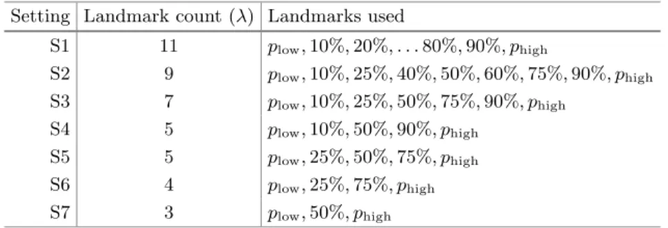
Seven different parameter setting schemes were defined, they are denoted by S1. . .S7, and listed in Table1. Each setting was involved in testing with values of plow varying between 1% and 5% in steps of 0.5%. The value ofphigh varied together withplowsuch a way that the equality phigh+plow= 100% was held.

Table 1.Various settings for the Approach A1 Setting Landmark count (λ) Landmarks used

S1 11 plow,10%,20%, . . .80%,90%, phigh

S2 9 plow,10%,25%,40%,50%,60%,75%,90%, phigh

S3 7 plow,10%,25%,50%,75%,90%, phigh

S4 5 plow,10%,50%,90%, phigh

S5 5 plow,25%,50%,75%, phigh

S6 4 plow,25%,75%, phigh

S7 3 p^low,50%, p^high

3.2 Method A2: Landmarks Established by Fuzzy c-Means

The second approach denoted by A2 employs a very similar mechanism as A1, but the landmark points are established by the use of the fuzzy c-means algo- rithm. The steps of the algorithm are presented in the following:

1. The previously defined target intensity interval is denoted by [α, β]. The num- ber of inner landmark points is set asλ≥2. In this study we evaluated cases with 2≤λ≤7.

2. A previously defined set of MRI records R is involved in the process, the number of records is denoted byr. The histogram of each record is extracted.

3. The set of landmark points is Λ ={plow, p_L1, p_L2, . . . , p_L,λ, phigh}, but only plow andphigh have predefined fixed values.

4. A first transformation step is performed: a linear transformation is designed such a way that maps y⁽_lowⁱ⁾ to y⁽_lowⁱ⁾ =α, y_high⁽ⁱ⁾ to y⁽_highⁱ⁾ =β, and applies this linear transform to all intensity values situated between y⁽ⁱ⁾_low and y_high⁽ⁱ⁾ in the original histogram. The two tails of the histogram is cut, meaning that intensity values belowy⁽ⁱ⁾_low are transformed toα, and intensity values above y_high⁽ⁱ⁾ are transformed toβ. For any j= 1. . . λ,y⁽_Ljⁱ⁾is transformed toy⁽_Ljⁱ⁾. 5. For all MRI records with indexi,i= 1. . . r, the transformed intensity values

undergo histogram-based quick fuzzyc-means clustering withc=λclusters.

The obtained cluster prototypes sorted in increasing order v1, v2, . . . v_λ are then assigned as dynamically established landmark points: y⁽_Ljⁱ⁾ = v_j∀j = 1. . . λ.

6. Target intensity values y_Lj for each inner landmark point with indexj (j= 1. . . λ) is computed next, using Eq. (1). These values are the same for all MRI records.

7. The target intensity values for the two extremes are:ylow=αandyhigh=β. 8. The final transformation is applied the same way as in the original A1 algo-

rithm, presented in Sect.2.3.

The algorithm is applied to each data channel separately.

3.3 Method A3: Linear Transform with One Parameter

The third approach denoted by A3 is a generalization of the technique proposed in our previous paper [21]. This method uses a single linear transformation, whose coefficients depend on the histogram of the original MRI volume. In con- trast with the previous two approaches, the normalization of any MRI record does not depend on other MRI records.

1. The previously defined target intensity interval is denoted by [α, β]. The algorithm uses a parameter q which controls the compactness of the final histogram.

2. The histogram of the current MRI record is extracted. The 25-percentile and 75-percentile intensity values are identified, and denoted byy25 andy75. 3. The target intensities for the 25-percentile and 75-percentile intensity values

are established using the formulas

y25=1 2

(β+α)−β−α q

and y75= 1 2

(β+α) +β−α q

. (3) 4. The coefficients of the linear transform y → ay+b are extracted such a way, thaty25andy75are transformed toy25andy75, respectively, using the formulas

a= β−α

q(y75−y25) and b=y25− (β−α)y25

q(y75−y25). (4) 5. Any intensity yfrom the input MRI volume becomes

y=

⎧⎨

⎩

α ifay+b < α ay+bifα≤ay+b≤β

β ifay+b > β . (5)

The algorithm is applied to each data channel separately. In our previous works [20–22], this approach was used with parameter settingq= 5.

4 Results and Discussion

Each of the three algorithms were tested with various settings using the same evaluation framework, having the target intensity interval bounded byα= 200 andβ= 1200, corresponding to an approximately 10-bit resolution. The 54 LGG

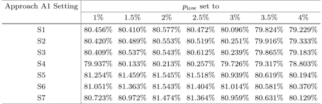
Table 2.Overall Dice scores obtained using Approach A1 using various settings

Approach A1 Setting plow set to

1% 1.5% 2% 2.5% 3% 3.5% 4%

S1 80.456% 80.410% 80.577% 80.472% 80.096% 79.824% 79.229%

S2 80.420% 80.489% 80.553% 80.519% 80.251% 79.916% 79.333%

S3 80.409% 80.537% 80.543% 80.612% 80.239% 79.865% 79.183%

S4 79.937% 80.133% 80.213% 80.257% 79.726% 79.317% 78.803%

S5 81.254% 81.459% 81.545% 81.518% 80.939% 80.619% 80.194%

S6 81.051% 81.363% 81.543% 81.404% 81.014% 80.581% 80.370%

S7 80.723% 80.972% 81.474% 81.364% 80.959% 80.631% 80.129%

Table 3.Overall Dice scores obtained using Approach A2 using various settings

Approach A2 Setting plow set to

1% 1.5% 2% 2.5% 3% 3.5% 4%

λ= 2 81.862% 82.122% 82.058% 81.991% 81.789% 81.561% 81.312%

λ= 3 81.829% 81.902% 81.958% 82.137% 81.857% 81.612% 81.105%

λ= 4 80.819% 81.494% 81.707% 81.789% 81.800% 81.548% 81.223%

λ= 5 79.289% 80.928% 81.150% 81.322% 81.077% 81.137% 81.085%

λ= 6 80.421% 80.426% 80.527% 80.732% 81.029% 81.012% 80.511%

λ= 7 80.965% 80.991% 80.668% 80.459% 80.722% 80.665% 80.722%

volumes of the BraTS 2016 data set underwent a ten-fold cross validation using the BDT ensemble based classifier algorithm described in Sect.2. Each ensemble consisted of 125 BDTs, each trained with 10000 randomly selected feature vectors from the train data, out of which 92% were negatives and 8% positives. From 104 generated features (for each of the 4 observed channels: minimum, maxi- mum and average extracted from 3×3×3 neighborhood; average and median extracted from planar neighborhoods of size ranging from 3×3 to 11×11; four directional gradients and eight directional Gabor wavelet values) the 13 most rel- evant features (minimum, maximum and average of T2 and FLAIR, maximum and average of T1C, and minimum of T1 from 3×3×3 neighborhood; average of T1C, T2 and FLAIR from 11×11 neighborhood; average of FLAIR from 3×3 neighborhood) were included into the feature vector, details are presented in our previous paper [22]. The outcome of the classification produced by the ensemble underwent a post-processing that relabeled each pixel according to the neighbors of the pixel. Those pixels were declared final positives, which had at least one third of its neighbors declared positive by the ensemble. The main evaluation criterion is the Dice score (DS), which is defined as DS = 2TP/(2TP+FP+FN), where TP, FP, and FN represent the number of true positives, false positives, and false negatives, respectively. Average Dice scores for each MRI record were established after the ten-fold cross-validation. Finally, the overall Dice score was

Table 4.Overall Dice scores obtained using Approach A3 using various settings

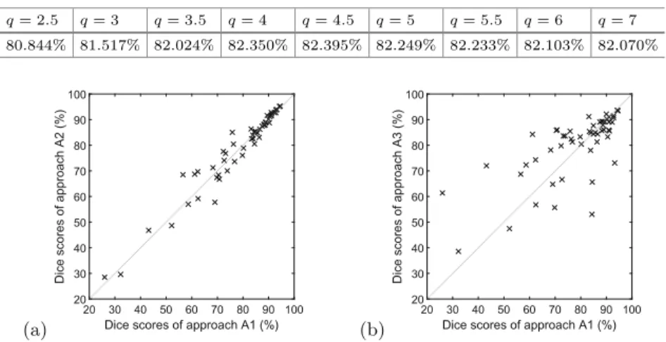
q= 2.5 q= 3 q= 3.5 q= 4 q= 4.5 q= 5 q= 5.5 q= 6 q= 7 80.844% 81.517% 82.024% 82.350% 82.395% 82.249% 82.233% 82.103% 82.070%

(a) 20 30 40 50 60 70 80 90 100Dice scores of approach A1 (%)

Dice scores of approach A2 (%)

20 30 40 50 60 70 80 90 100

(b) 20 30 40 50 60 70 80 90 100Dice scores of approach A1 (%)

Dice scores of approach A3 (%)

20 30 40 50 60 70 80 90 100

Fig. 2.Dice scores obtained on individual LGG records, the best performance of the three approaches plotted one against another: (a) A2 vs. A1; (b) A3 vs. A1.

computed for each approach and setting, based on all pixels from all volumes.

Results are exhibited in Tables2,3 and4.

The best achieved overall Dice score (ODS) is 82.395%. Most of the evaluated approaches and settings led to ODS values over 80%. The classical A1 approach hardly achieved 81.5%, with its best setting that used the landmark set{plow= 2%,25%,50%,75%, phigh= 98%}, where the middle landmark point is virtually optional. A larger number of landmarks, as used for example in [17,18], in our studies led to ODS around 80.5%, which is well below optimal.

The A2 approach achieved best ODS values around 82%, when using 2 or 3 inner landmarks,plowranging between 1.5% and 2.5%. The accuracy is finer than in case of approach A1, while the best scenario is quite similar.

The A3 approach has a wide interval of its parameter, where the algorithm scores ODS values above 82%. The best accuracy was achieved atq= 4.5, which means that in each data channel of the MRI records, all original intensity values are subject to linear transformation into the target interval [200,1200] such a way, that the 25-percentile is mapped to 578, the 75-percentile to 822, and the tails of the transformed histogram is cut at 200 and 1200. The normalization of any histograms occurs independently, it does not depend on the histograms of other records or other data channels.

Figure2 exhibits the comparison of the three approaches, when applied to individual MRI volumes. Each approach is represented with its overall best set- ting. This figure also shows that A3 and A2 can perform slightly better than A1, but the slight superiority comes in average only, because the segmentation accuracy of individual MRI records can be either better of worse, with virtually same probability. Tests have confirmed the observation of Tustison et al. [19], who remarked that a well designed simple linear transformation performs better

than previous algorithms like A1, in such tumor segmentation problems. Fur- ther tests involving more data, more algorithms, and further quality indicators could provide stronger evidence of this superiority. Our results do not mean that A3 leads to better accuracy than the frequently used A1 in all segmentation problems. But when the goal is tumor detection, it is recommendable to apply histogram normalization via approach A3.

5 Conclusions

This study investigated the effect of various histogram normalization methods upon the final accuracy in an MRI data based brain tumor segmentation prob- lem. Two approaches were proposed and compared to the most frequently used and most cited such algorithm. Tests have revealed a slight superiority of both proposed algorithms, compared to the previous one.

References

1. Ny´ul, L.G., Udupa, J.K., Zhang, X.: New variants of a method of MRI scale stan- dardization. IEEE Trans. Med. Imaging19(2), 143–150 (2000)

2. Weisenfeld, N.L., Wartfeld, S.K.: Normalization of joint image-intensity statistics in MRI using the Kullback-Leibler divergence. In: IEEE International Symposium on Biomedical Imaging (ISBI), pp. 101–104. IEEE (2004)

3. J¨ager, F., Deuerling-Zheng, Y., Frericks, B., Wacker, F., Hornegger, J.: A new method for MRI intensity standardization with application to lesion detection in the brain. In: Kobbelt, L., et al. (eds.) Vision Model, Visualization, pp. 269–276.

AKA GmbH, K¨oln, Germany (2006)

4. Leung, K.K., et al.: Robust atrophy rate measurement in Alzheimer’s disease using multi-site serial MRI: tissue-specific intensity normalization and parameter selec- tion. Neuroimage50, 516–523 (2010)

5. Shinohara, R.T., Crainiceanu, C.M., Caffo, B.S., Gait´an, M.I., Reich, D.S.:

Population-wide principal component-based quantification of blood-brain-barrier dynamics in multiple sclerosis. Neuroimage57(4), 1430–1446 (2011)

6. Pereira, S., Pinto, A., Alves, V., Silva, C.A.: Deep convolutional neural networks for the segmentation of gliomas in multi-sequence MRI. In: Crimi, A., Menze, B., Maier, O., Reyes, M., Handels, H. (eds.) BrainLes 2015. LNCS, vol. 9556, pp.

131–143. Springer, Cham (2016).https://doi.org/10.1007/978-3-319-30858-6 12 7. Meier, R., et al.: Clinical evaluation of a fully-automatic segmentation method for

longitudinal brain tumor volumetry. Sci. Rep.6, 23376 (2016)

8. Ellwaa, A., et al.: Brain tumor segmantation using random forest trained on iter- atively selected patients. In: Crimi, A., et al. (eds.) BrainLes 2016. LNCS, vol.

10154, pp. 129–137. Springer, Cham (2017). https://doi.org/10.1007/978-3-319- 55524-9 13

9. Bakas, S., et al.: Advancing the cancer genome atlas glioma MRI collections with expert segmentation labels and radiomic features. Sci. Data4, 170117 (2017) 10. Rezaei, M., et al.: A conditional adversarial network for semantic segmentation

of brain tumor. In: Crimi, A., Bakas, S., Kuijf, H., Menze, B., Reyes, M. (eds.) BrainLes 2017. LNCS, vol. 10670, pp. 241–252. Springer, Cham (2018).https://

doi.org/10.1007/978-3-319-75238-9 21

11. Fidon, L., et al.: Scalable multimodal convolutional networks for brain tumour segmentation. In: Descoteaux, M., Maier-Hein, L., Franz, A., Jannin, P., Collins, D.L., Duchesne, S. (eds.) MICCAI 2017. LNCS, vol. 10435, pp. 285–293. Springer, Cham (2017).https://doi.org/10.1007/978-3-319-66179-7 33

12. Chen, X., Nguyen, B.P., Chui, C.K., Ong, S.H.: An automated framework for multi-label brain tumor segmentation based on kernel sparse representation. Acta Polytech. Hung.14(1), 25–43 (2017)

13. Soltaninejad, M., Zhang, L., Lambrou, T., Yang, G., Allinson, N., Ye, X.: MRI brain tumor segmentation and patient survival prediction using random forests and fully convolutional networks. In: Crimi, A., Bakas, S., Kuijf, H., Menze, B., Reyes, M. (eds.) BrainLes 2017. LNCS, vol. 10670, pp. 204–215. Springer, Cham (2018).https://doi.org/10.1007/978-3-319-75238-9 18

14. Chen, W., Liu, B.Q., Peng, S.T., Sun, J.W., Qiao, X.: Computer-aided grading of gliomas combining automatic segmentation and radiomics. Int. J. Biomed. Imaging 2018, 2512037 (2018)

15. Wu, Y.P., Liu, B., Lin, Y.S., Yang, C., Wang, M.Y.: Grading glioma by radiomics with feature selection based on mutual information. J. Ambient Intell. Hum. Com- put.9(5), 1671–1682 (2018)

16. Chang, J., et al.: A mix-pooling CNN architecture with FCRF for brain tumor segmentation. J. Vis. Commun. Image Represent.58, 316–322 (2019)

17. Soltaninejad, M., et al.: Supervised learning based multimodal MRI brain tumour segmentation using texture features from supervoxels. Comput. Methods Programs Biomed.157, 69–84 (2018)

18. Pinto, A., Pereira, S., Rasteiro, D., Silva, C.A.: Hierarchical brain tumour segmen- tation using extremely randomized trees. Pattern Recogn.82, 105–117 (2018) 19. Tustison, N.J., et al.: Optimal symmetric multimodal templates and concatenated

random forests for supervised brain tumor segmentation (simplified) with ANTsR.

Neuroinformatics13, 209–225 (2015)

20. Lefkovits, L., Lefkovits, S., Szil´agyi, L.: Brain tumor segmentation with optimized random forest. In: Crimi, A., et al. (eds.) BrainLes 2016. LNCS, vol. 10154, pp.

88–99. Springer, Cham (2017).https://doi.org/10.1007/978-3-319-55524-9 9 21. Szil´agyi, L., Icl˘anzan, D., Kap´as, Z., Szab´o, Z., Gy˝orfi, ´A., Lefkovits, L.: Low

and high grade glioma segmentation in multispectral brain MRI data. Acta Univ.

Sapientia Informatica10(1), 110–132 (2018)

22. Gy˝orfi, ´A., Kov´acs, L., Szil´agyi, L.: A feature ranking and selection algorithm for brain tumor segmentation in multi-spectral magnetic resonance image data. In:

41st Annual Conference of the IEEE EMBS. IEEE (2019, accepted paper) 23. Bezdek, J.C.: Pattern Recognition with Fuzzy Objective Function Algorithms.

Plenum, New York (1981)

24. Menze, B.H., Jakab, A., Bauer, S., Kalpathy-Cramer, J., Farahani, K., Kirby, J., et al.: The multimodal brain tumor image segmentation benchmark (BRATS).

IEEE Trans. Med. Imaging34, 1993–2024 (2015)

25. Bakas, S., Reyes, M., Jakab, A., Bauer, S., Rempfler, M., Crimi, A., et al.:

Identifying the best machine learning algorithms for brain tumor segmentation, progression assessment, and overall survival prediction in the BRATS challenge.

arXiv: 1181.02629v3, 23 April 2019