Párhuzamos, lokális módszerek vizsgálata a képszegmentálásban, tömörítésben és optikai mozgásanalízisben

Ph.D. Thesis of Czúni László

Supervisor: Szirányi Tamás MI 1 Ph.D. Program University of Veszprém

2000

mozgásanalízisben

(Analysis of Parallel Local Methods in Image Segmentation, Image Compression, and Motion Analysis)

Értekezés doktori (Ph.D.) fokozat elnyerése érdekében

Írta: Czúni László informatikus mérnök

.pV]OWD9HV]SUpPL(J\HWHP0 V]DNL,QIRUPDWLNDGRNWRULSURJUDPHV0,MHO alprogramja keretében.

7pPDYH]HW 'U6]LUiQ\L7DPiV Elfogadásra javaslom: igen / nem .

………

dátum, aláírás

A jelölt a doktori szigorlaton ……%-ot ért el.

Veszprém, 200………

………...

a Szigorlati Bizottság elnöke

Az értekezést bírálóként elfogadásra javaslom: igen / nem . Els bíráló: ………. igen / nem

………

aláírás

Második bíráló: ………. igen / nem

………

aláírás

A jelölt az értekezés nyilvános vitáján ……%-ot ért el.

Veszprém, 200………

………...

a Bíráló Bizottság elnöke

$GRNWRUL3K'RNOHYpOPLQ VtWpVH««««««

………...

az EDT elnöke

TABLE OF CONTENTS

KIVONAT... 1

ABSTRACT ... 2

ZUSAMMENFASSUNG... 3

RELATED PUBLICATIONS ... 4

PREFACE: PARALLEL ARCHITECTURES AND CELLULAR ARRAYS... 7

CHAPTER I

2 MRF IMAGE SEGMENTATION MODELS WITH MAXIMUM A POSTERIORI OPTIMIZATION ... 10

2.1 BASIC DEFINITIONS... 10

2.2 THE SEGMENTATION MODEL: BAYESIAN MODEL WITH MAXIMUM A POSTERIORI (MAP) ESTIMATION... 12

2.3 THE ENERGY FUNCTION... 13

2.4 OPTIMIZATION BY MODIFIED METROPOLIS DYNAMICS (MMD)... 14

3 THE CNN-MRF SEGMENATION MODELS... 16

3.1 PARALLEL SOLUTION ON THE CNN... 16

3.2 A MONOGRID CNN-MRF MODEL BASED ON LOCAL STATISTICS... 19

3.3 EXPERIMENTS WITH THE MONOGRID CNN-MRF MODEL... 22

3.4 NONLINEAR DIFFUSION FOR DETAIL CONSERVATION... 23

3.5 MULTIGRID MODELS... 24

3.6 THE CNN-MRF MULTISCALE MODEL... 26

3.7 EXPERIMENTS WITH THE MULTIGRID CNN-MRF MODEL... 28

3.8 CHARACTERISTICS OF THE IMPLEMENTED MODELS: COMPARING MONOGRID AND MULTIGRID CNN-MRF MODELS... 32

3.9 THE ROBUSTNESS OF THE CNN-MRF MODEL ON IMPRECISE ANALOG CIRCUITS... 32

4 CONCLUSIONS... 42

CHAPTER II

IMAGE COMPRESSION WITH NOISY 2D PROCESSOR ARRAYS

1 INTRODUCTION...43

1.1 A PARALLEL IMAGE CODING MODEL IN THE CNN ENVIRONMENT...44

1.2 THE BASIC CNN CHIP-SET...45

1.3 THE ARCHITECTURE OF THE ORTHOGONAL ANALYZER AND DECODER...45

1.4 THE PROCESSING CYCLE...48

1.5 COMPUTATION TIMES...51

2 CODING IN A NOISY COMPUTATION MODEL...54

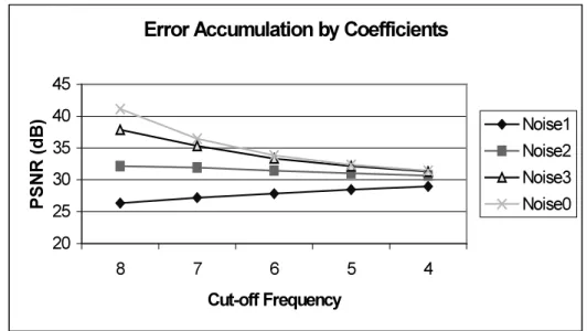
2.1 THE EFFECT OF A/D CONVERSION AND THE ACCUMULATION OF COEFFICIENT INACCURACY...56

2.2 THRESHOLDING COEFFICIENTS...59

2.3 PARAMETERS FOR THE COMPRESSION OF AN IMAGE BLOCK...63

3 OPTIMIZING THE COMPRESSION IN A DYNAMIC CODING ENVIRONMENT ...64

3.1 DYNAMIC IMAGE CODING WITH LAGRANGE OPTIMIZATION...64

3.2 OPTIMAL IMAGE CODING WITH LAGRANGE OPTIMIZATION IN QUADTREE REPRESENTATION...65

3.3 ANALYSIS OF CODE EFFICIENCY...68

4 CONCLUSIONS...75

CHAPTER III

1.1 GENERAL TASKS IN MOTION SEGMENTATION AND TRACKING... 80

1.2 BASIC FEATURES OF THE PROPOSED CNN-BASED MODEL... 81

1.3 ELEMENTARY FUNCTIONS OF THE CELL ARRAY... 83

2 ESTIMATION AND SEGMENTATION OF THE OPTICAL FLOW... 84

2.1 ESTIMATION OF THE MOTION DISPLACEMENT FIELD... 84

2.2 MOTION ESTIMATION BY A PARALLEL CORRELATION TECHNIQUE... 85

2.3 SEGMENTATION WITH AN MRF-BASED METHOD... 88

2.4 A GRADIENT-BASED METHOD: SIMULTANEOUS ESTIMATION AND SEGMENTATION OF THE OPTICAL FLOW BY ENERGY MINIMIZATION... 91

2.4.1 Constraints for the Optical Flow from the Intensity Conservation ... 92

2.4.2 Segmentation by Energy Minimization... 93

2.4.3 Related Motion Segmentation Models Based on Energy Minimization ... 95

3 EDGE OPTIMIZATION FOR SPATIO-TEMPORAL SEGMENTATION AND TRACKING... 96

3.1 SUBROUTINES OF THE PROPOSED MODEL... 96

3.1.1 Nonlinear Diffusion... 96

3.1.2 Pixel Level Tracking: Motion History... 97

3.1.3 Morphology Operators on Cell Arrays ... 98

3.1.4 Disocclusion Removal in Parallel... 98

3.2 THE BASIS OF THE SPATIO-TEMPORAL SEGMENTATION ALGORITHM... 99

3.3 THE SEGMENTATION PROCESS... 100

4 EXPERIMENTAL RESULTS ... 106

5 VLSI CHIP SPEED AND COMPLEXITY ESTIMATION ... 110

6 CONCLUSION... 112

THESES ...113

ACKNOWLEDGEMENTS...116

REFERENCES ...117

Kivonat

$ MHOHQ GRNWRUL pUWHNH]pV D NpSIHOGROJR]iV KiURP NO|QE|] WHUOHWpQHN KiURP speciális részterületével foglalkozik:

• statisztikai képszegmentálás - képanalízis,

• DCT (Diszkrét Koszinusz Transzformáció) alapú képtömörítés – képkódolás,

• PR]JiVV]HJPHQWiOiVV U YHNWRUPH] N|Q±PR]JiVDQDOt]LV

$ GROJR]DWEDQ WiUJ\DOW DOJRULWPXVRN PLQGHJ\LNH DODSYHW HQ DEEDQ NO|QE|]LN D]

irodalomban eddig található eljárásoktól, hogy ezek párhuzamos processzortömbökre lettek kidolgozva. Míg az ilyen platformoknak nagyon jó az ár/teljesítmény mutatója, DGGLJ V]iPRWWHY D] D KiWUiQ\XN KRJ\ FVDN PHJKDWiUR]RWW WtSXV~ pV V]iP~

P YHOHWHNUH NpSHVHN NRUOiWR]RWW D ORNiOLV PHPyULiN V]iPD pV QHP W~O QDJ\ D számítási pontosságuk (~8bit).

$] HOV IHMH]HWEHQ HJ\ 0DUNRY 9DOyV]tQ VpJL 0H] Q 0DUNRY 5DQGRP )LHOG MRF) alapuló szegmentálási eljárás a vizsgálat tárgya, tekintettel a többfelbontásos megvalósításra. A fejezet külön kitér a számítási zaj hatására, ami – egy bizonyos pUWpNDODWWDV]WRFKDV]WLNXVRSWLPDOL]iOiVLPyGQDNN|V]|QKHW HQQHPURQWMDKDQHP javítja a szegmentálási teljesítményt.

A számítási zaj szintén fontos szerepet játszik a második fejezetben is, ahol egy RUWRJRQiOLV WUDQV]IRUPiFLyW YpJ] DUFKLWHNW~UD D V]iPtWiVRN DODSMD ,WW HJ\

optimalizáló kódolási stratégia biztosítja a hatékony tömörítést a zajos áramkörökön, akár több transzformációs eljárás segítségével (Koszinusz és Hadamard transzformációk).

0R]JiV pV WpULG EHOL V]HJPHQWiOiVL HOMiUiVRNNDO IRJODONR]LN D KDUPDGLN IHMH]HW $ mozgásvektor szegmentálási eljárások MRF alapú statisztikai módszerekkel P N|GQHNPtJDWpULG EHOLHOMiUiVSL[HOV]LQW N|YHWpVWWpUEHOLLQWHQ]LWiVLQIRUPiFLyW pV D] HO ] OHJ EHFVOW PR]JiVPH] W KDV]QiOMD D PR]Jy IROWRN REMHNWXPRN MREE szegmentálása érdekében.

Abstract

The Thesis deals with three topics of three main areas of image processing:

• statistical image segmentation (image analysis)

• DCT (Discrete Cosine Transformation) based image compression (image coding)

• motion segmentation (based on dense vector field) (motion analysis).

All the discussed methods differ from most of the preceding algorithms found in literature by the fact that they are supposed to run on fully parallel processor arrays.

While these platforms, when realized in VLSI chips, have superior computational speed at relatively low cost compared to other architectures, have the disadvantage of restricted number and type of operations, number of memory and precision of computations.

In Chapter I a Markov Random Field (MRF) based image segmentation method is investigated also in view of multiscale implementation. Some important observations of this chapter come from simulations of computation noise, which show that a certain amount of noise even enhances the segmentation performance, thanks to the stochastic optimization technique.

The effect of computation noise also plays important role in Chapter II, where compression architecture, based on orthogonal decomposition, is described.

Furthermore a bit allocation strategy is proposed based on the competition of Hadamard and Discrete Cosine Transformations.

Motion and spatio-temporal segmentation algorithms are discussed in Chapter III.

Motion vector segmentation methods are based on MRF statistical methods, while the spatio-temporal segmentation algorithm uses a pixel-level tracking algorithm, the spatial intensity information and the estimated motion field for a better segmentation of moving blobs in an image sequence.

Zusammenfassung

Die Arbeit beschäftigt sich mit drei Teilgebieten der Bildvearbeitung:

• Statistische Bildsegmentierung (Bildanalyse)

• Einfluß der DKT (Diskret Kosinus Transformation) auf die Bildkompression – Bildcodierung

• Bewegung-Segmentierung (basierend auf dichten Vektorfeldern) – Bewegungsanalyse

Alle Algorithmen dieser Arbeit unterscheiden sich von den Algorithmen die in der Literatur beschrieben wurden dadurch, dass diese Algorithmen für Paralellmatrixrechner ausgearbeitet worden sind. Diese Hardwerbasis besitzt ein sehr gutes Kosten/Rechenegeschwindigkeitverhältsnis, aber es hat auch mehrere Nachteile.

Das eine ist die eingeschränkte Zahl und Art von Operationen, das zweite ist die begrenzte Zahl der Arbeitsspeicher und Rechengenauigkeit.

Im ersten Kapitel wird eine auf dem Markov Random Field beruhende Segmentierungsmethode untersucht, es wird auch die multiscale Implementation beabsichtig. Einige wichtige Beobachtungen dieses Kapitels kommen von der Simulation des Rechnerrauschens. Es wird gezeigt, dass ein gewisses Mass von Rechnerrauschen sogar zur Erhöhung der Segmentationsgüte beiträgt. Dies ist der stochastischen Optimierungstechnik zu danken.

Das Rechnenrauschen hat eine wichtige Rolle auch im zweiten Kapitel, wo eine Kompressionsarchitektur beschrieben wird, die auf eine orthogonale Zerlegung basiert. Hier wird auch eine Strategie der Bit-Zuordnung vorgeschlagen, die auf Hadamard und Diskret Kosinus Transformation beruht.

Bewegungs- und RaumzeitSegmentierungsalgoritmen werden im dritten Kapitel untersucht. Der Algoritmus der Bewegungsvektorsegmentierung basiert auf einen MRF statistischen Algoritmus, während der Raumzeitalgoritmus das Nachführen des Bildpunkt-Niveaus benutzt, es benutzt die Helltasten der Information in dem Raum und dem Bewegungsfeld für bessere Segmentierung der Bewegung Flecken in einer Bildsequenz.

Related Publications

While the Thesis has three main chapters dealing with different areas of image processing, they are all common that they are related to image coding and use the same architecture for computations. This platform can be described as a fully parallel architecture consisting of cell elements generally organized in matrix form. These elements are connected to each other, contain memory and processing units and usually represent image pixels. One typical example for these platforms is the analog Cellular Neural/Nonlinear Network (CNN) [14,77], while other digital devices also exist such as the Mitshubishi’s artificial retina [99] or other smart pixel arrays [24].

Currently, according to its physical parameters and complexity [21,57] it seems that CNN is capable of the most complex computations, however, it is also true that for certain applications other (even 1D) architectures are also satisfactory [82].

Chapter I contains algorithms for image segmentation based on Markov Random Fields (MRFs). General reviews of image segmentation can be found in [34,64], however, the application of MRF techniques in image analysis and segmentation are in [4,8,9,10, 20,30,32,35,47,49,50,51,104]. According to a large number of publications in this field, algorithms described in the Thesis differ in the basic interpretation of data of observations made at pixel locations [96]. This is necessary for the localization of statistical features (expected value and variance are measured at the pixel-level instead of using global classes) and makes the CNN adaptation possible. Also none of the known literature deals with the realization of MRF related statistical algorithms on noisy hardware. The described models of the Thesis also seem to be good applications of the so-called Modified Metropolis Dynamics (MMD) optimization method [50], what is a special type of Simulated Annealing [30,52], while multiscale MRF segmentation methods have been tested according to [32].

Chapter II deals with the possible use of CNN in image compression. While there are a lot of papers about the application of CNN in image processing and a lot of papers in the area of general image coding, only a very few articles deal with image coding/compression in the CNN environment. In [100,101] an architecture for DCT (Discrete Cosine Transform) and subband-based compression are given, however, the Thesis proposes a different architecture capable of simultaneous coding and decoding of the image [94]. This feature is necessary to implement Shannon’s rate-distortion theory [83], a framework that is used to choose an optimal bit allocation strategy. It is also important to mention that while CNN seems to be quite robust in MRF-based segmentation, it is a bigger problem in image coding where the effect of computational noise can decrease image quality seriously. While [100,101] do not deal with the effects of noise, it is discussed in the current paper in details. Many other

bit allocation strategies exist (e.g. [15,59]), the currently most used one (based on DCT) is JPEG [105]. In the Thesis a different algorithm for optimal bit allocation is proposed, it is similar to the Dynamic Video Coding (DVC) approach discussed in [22,72]. [25] describes the algorithmic solution for converting constraint problems to unconstrained problems, also used in the proposed optimization algorithm.

In Chapter III motion segmentation algorithms and a spatio-temporal segmentation algorithm is proposed. These algorithms can serve as bases for second generation image/video coding. [98] contains details about this approach considered as a successor of today’s compression technology [43,44,46], while MPEG-4 [45] is already one main application of this technique.

Several optical flow estimation and segmentation techniques have been investigated from the aspects of parallel implementation. [6,7,55,58,88] serve as good starting points for comparisons of computation complexity and performance of several methods.

Correlation-based techniques are widely used in MPEG applications but their serial implementation is very time consuming. In case of motion field optimization, iterative or relaxation algorithms are used to obtain reliable results [40,65]. However, the iterative reevaluation of the displaced frame difference increases time complexity and may not fit our computation model based on local interactions. Generally, correlation techniques seem to be rejected in the Simple Instruction Multiple Data (SIMD) model we addressed, but now we show that if no motion model based optimization is needed then our fully parallel architecture can compute vector estimates with the correlation technique.

According to [6] gradient-based approaches have good accuracy, although, it is also well-known that these methods are very sensitive to temporal aliasing and need large temporal support. In [6] best results needed 15 image frames to be stored in memory simultaneously for computations (see the next section). In [28] a recursive filter is designed to avoid the need for large image memories and long delays, and they report similar results to the original model in accuracy.

In [84] filter banks had been built for spatio-temporal filtering. Their method is well suited for parallel implementation and has good accuracy as reported, but its application could be limited due to the large number of filters needed for general image flows.

[49] describes motion compensated vector classification in the MRF framework. The proposed model in [49] applies 3D cliques to exploit inter-frame information, but this method still leads to color classification instead of real spatio-temporal segmentation, which is closer to the recognition of video objects.

Many probabilistic approaches use region labeling algorithms for spatio-temporal segmentation, e.g. [11,31]. These models, however, can not be implemented in our parallel framework, since the proposed region indexing and labeling methods are not well suited to the pixel array with many similar local processing elements and memories. That is why a different contour-based segmentation method is employed in this work.

Besides this overview other observations and comparisons are present in the following three Chapters.

P

: P

A

C

A

While in the past a lot of effort has been made to design real-time hardware systems, today many of those problems can be solved with high performance general-purpose personal workstations at low cost. On the other hand there is an increasing demand for a new generation of image analysis tasks, such as second-generation video coding [62,98], virtual reality, etc. While up-to-date Complex Instruction Set Computers (CISC), such as PCs based on the Pentium MMX family, speed up multimedia applications tremendously, these tasks are still far from being in the range of the computing power of conventional CISC machines in the close future [58,70].

One possible breakthrough is the use of cellular processor arrays (analog or digital) which assign a simple processor to each pixel resulting in fully parallel operation [14,77]. Contrary to the general CISC class of processors, which can also show some parallel capabilities as well, cellular processor arrays can utilize only simple pixel based functions defining a relatively narrow instruction set – although, at a very high speed.

The typical example for the higher cell-complexity of cellular processor arrays is the family of the Cellular Neural/Nonlinear Network (CNN) chips [21,57]. CNN can process images locally on the pixel-level with small neighborhood connectivity. It can perform convolution, nonlinear (sigmoid) dynamics, etc. in a feed-forward/feed-back operation mode. CNN Universal Machine (CNN-UM) [77] is a programmable computer based on the basic CNN architecture with many additional features like those that conventional computers have: local and global memories, pixel-level logical and arithmetic functions, digital memories etc., all in one single chip.

Investigating the success of general-purpose high performance processors in the image processing area, it seems to be reasonable to develop new, low-level algorithms for this new class of cellular processor arrays, since they can be considered as widely usable real-time image processing architectures with superior speed, integrated into VLSI. The crucial question is how to develop a successful cellular image processing system for certain purposes containing local connections and reduced instruction set, considering the limitations of the cell-complexity of VLSI implementation

CHAPTER I

M

R

F

-B

I

S

A

P

A

1 I

S

Image segmentation can be considered as a special kind of image classification. In dense pixel classification pixels are represented in the feature space and in many cases the task is to find the most important feature vector elements that are required to group the pixels into classes. A very important aspect in segmentation is that the spatially neighboring pixels should belong to the same class with high probability.

Image segmentation is an operation very often used in image processing. Its output can be directly useful to a large class of applications such as medical image processing, agricultural applications, etc. High level applications, such as robot vision and second generation image coding also use segmentation as an essential low-level preprocessing step.

There are a large number of different image segmentation algorithms [34,64]. The most important criteria for good segmentation are the following:

• The segmented image should contain connected and disjoint regions.

• All pixels should belong to one class.

• Regions should be homogenous with well-defined contours separating them.

However, it is always a question how to evaluate an image segmentation algorithm. In most cases artificially generated images serve as ground truth. In cases of natural data the image is usually segmented manually, based on auxiliary information, and the result obtained is used for performance evaluation of the automatic segmentation process.

Many of the segmentation methods, e.g. split and merge, region growing, etc., construct a graph (or similar high-level) representation of the image content.

Unfortunately, this kind of high-level representation is not possible in our framework where images are represented densely on a lattice of elements. The most important feature of the Markov Random Field (MRF)-based segmentation models discussed in this chapter is that they are based on low level observations and operations. On the

other hand, a very important aspect of the development of the following algorithms was to use simple operations that are realizable in analog VLSI circuits.

The proposed low-level processes can be used for the segmentation of grayscale, non- textured images. Such kinds of images are common in medical image processing (e.g.

Computer Tomography (CT) and Magnetic Resonance Imaging (MRI) data) or in the area of processing spot or air-born images.

A very important feature of the presented algorithms that they can be executed parallel promising a fast VLSI implementation on cell array computers such as the CNN-UM.

2 MRF I

S

M

M

A P

O

Since the work of Geman and Geman [30] there are a lot of examples where stochastic optimization and Bayesian approaches are used for solving image labeling problems. However, the idea of parallel, low-level cooperating processes is much older, many basic ideas were already reviewed in [20]. Examples for edge detection, image segmentation, restoration, stereovision, motion segmentation, etc. can be found in [4,8,9,10,30,32,35,50, 51,104].

For many of the early vision processes, where the image is represented on a lattice, the problem is posed as a labeling problem. In our case, when our aim is to segment the input image to a given number of classes, we will determine the possible classes by the grayscale information of the input image, but usually MRF based methods can be extended to the analysis of color images as well [47,49].

To find an optimal labeling, the minimization of a cost function - which is constructed from the observed data, a priori information and constraints - is needed. The obtained cost function is usually non-convex and several relaxation techniques have been proposed to reach an optimum labeling. One class of methods deals with stochastic relaxation and is based on Simulated Annealing (SA) [30,52]. These algorithms converge asymptotically towards the global minimum but require a great deal of computation. The second group of methods is related to deterministic relaxation.

These techniques are sub-optimal but require less computational time than the previous ones. That is why so many deterministic (or pseudo stochastic) relaxation algorithms have been recently investigated (Graduated Non Convexity (GNC) [9], Iterated Conditional Mode (ICM) [8], Mean Field Annealing (MFA) [104], Modified Metropolis Dynamics (MMD) [50]). In the proposed framework the MMD will be implemented.

2.1 Basic Definitions

First, I give a brief introduction to the theory of MRF [3,74,96], and then a general image model, used in the following sections, is described.

Let )S=(s₁,s₂,s₃,...s_N be a set of sites (or pixels). Two points s_i and s_j are neighbors, if there is an edge connecting them. The set of points that are neighbors of site s is denoted G_s. G⁼

{

}

1. s∉G_s

2. s∈G_r ⇔r∈G_s.

A subset C ⊆S is a clique if every pair of distinct sites in C is composed of two neighbors. C denotes the set of all cliques. In image processing the most commonly used neighborhood systems are the homogeneous systems. In this case, we consider S as a lattice and define these neighborhoods as

{

}

= ₍ⁿ_i,j):(i,j)

n G

G ,

{

}

n j

i, ) = ∈ − ² + − ² ≤

( ( , ) S:( ) ( )

G .

Obviously, sites near the boundary have fewer neighbors than interior ones.

Furthermore, G⁰ ≡S and for all n≥0:Gⁿ ⊂Gⁿ⁺¹. Fig. 1 shows a first-order neighborhood corresponding to n=1. The cliques are {(i,j)}, {(i,j), (i,j+1)}, {(i,j), (i+1,j)}.

Let X =

{

}

{

}

Furthermore, let Ω=

{

}

3 2

1 ω ω ω ω

ω

ω be the set of all

possible configurations.

X is a MRF with respect to Gif 1. ∀ω∈Ω:^P(^X =ω)>0,

2. ∀s∈^S,∀ω∈Ω:P(X_s =ω_s |X_r =ω_r,r≠s)=P(X_s =ω_s|X_r =ω_r,r∈G_s).

A central site and its 4 neighbors Cliques Figure 1.

First order neighborhood-system and cliques.

The functions in point 2 are called the local characteristics of the MRF, and the probability distribution P(X =ω) of any process, satisfying point 1, is uniquely determined by these conditional probabilities. However, it is extremely difficult to determine these characteristics in practice. Gibbs distribution and the Hammersley- Clifford theorem provide us a simple way to solve this problem.

A Gibbs distribution, relative to the neighborhood system G, is a probability measure π on Ω with the following representation:

(

)

1exp )

(ω ω

π ^E

Z −

= (1)

where Z is the normalizing constant or partition function:

( )

∑

=

ω exp E(ω)

Z , (2)

and the energy function E is of the form:

∑

=

C C

EC

E(ω) (ω). (3)

Each E_C is a function defined on Ω depending only on those ωs elements of ω for which s∈C. The restriction of ω to the sites of a given clique C is denoted by ωC. Such a function is called a potential. A very important theorem is the Hammersley- Clifford theorem, which points out the relation between the MRF and the Gibbs distribution:

• X is a MRF with respect to the neighborhood system G if and only if )

( )

(ω ω

π =P X = is a Gibbs distribution with respect to G.

Using the above theorem the definition of the MRF is completed by the knowledge of the clique potentials E_C(ω_C) for every C in C and every ω in Ω.

2.2 The Segmentation Model: Bayesian Model with Maximum A Posteriori (MAP) Estimation

During the labeling segmentation process we would like to choose the most probable labels, i.e. our estimation should be based on the Bayesian estimation model. We can start from the following probabilities:

) (

) ( )

| ) (

|

( P F

P F F P

Pω = ω ω , (4)

where F is the observed grey-level image data, F =

{ }

) ( 1 )

’ ,

(ω ω = −Δω_’ ω

R , (5)

where )Δω_’(ω is the Dirac mass at ω =ω’. The Bayes risk to be minimized is:

{

}

E ω , (6)

where d is a decision function based on our observations. Considering that F is constant in our model and combining the above equations we get:

) ( )

| ( max arg )

| ( max arg )

| ( )

’ , ( min

arg ’ ω ω ω ω ω ω ω

ω_OPT ω ω R P F d ω P F ω P F P

Ω

∈ Ω

Ω ∈

∈ Ω

∈ = =

=

∫

(7) Now, utilize the Hammersley-Clifford theorem to substitute P(ω) probabilities with energy potentials and write the above equation in the following form:

( )

∏ −

= ∏

∈ Ω ∈

∈ S C C C

s s s

OPT argmax P(f |ω ) exp E (ω)

ω ω . (8)

2.3 The Energy Function

Taking the logarithm of Eq. (8) and assuming that P(f_s|ω_s) is Gaussian we can formulate an energy function:

) ( ) , ( ) ,

(ω F = E₁ ω F +E₂ ω

E , (9)

where

∈∑

+ −

= S s

f

s s s

F s

E

ω ω

ω σ

σ μ

ω π ₂

2 )2 ) (

2

) ln(

,

1( , (10)

= ∑

∈C

C EC

E₂(ω) (ω), (11)

{ } ⎩⎨⎧

≠

=

= −

=

r s

r s r

s r s

C if

E if

E β ω ω

ω ω ω β

ω ω) ( , )

( _, , (12)

(This last one is a penalty function to encourage homogeneity of labels ωs and ωr in cliques).

That is to find an optimum solution for the Bayesian estimation problem (Eq. (8)) we can run an energy optimization algorithm during which we are to get the smallest energy E (Eq. (9)) over the lattice S.

A basic assumption in image segmentation is that the observed input image can be well characterized by a finite number of classes. Within a Gaussian model each class can be represented by its mean value μ and by its standard deviation σ. That is each possible label should have its appropriate mean μλ and deviation σλ. The first energy term (E₁) is responsible to keep the labeling close to observations, while the second energy term (E₂) is to achieve fairly homogenous regions, which is an important requirement in image segmentation. β is a positive model parameter controlling the homogeneity of regions of the segmented image. Typically, small β retains little image segments, while larger β causes the formation of larger regions. For more details of more general image models the reader should refer to [50, 56].

2.4 Optimization by Modified Metropolis Dynamics (MMD)

During the relaxation process, new random labels (also called states) are generated in each iteration and compared to the previous labels. Labels are compared on the basis of the already defined energy function (Eq. (9)), however, the decision criteria can vary according to the optimization algorithm.

Basically, the MMD algorithm [50] is a modified version of Metropolis Dynamics [60] and it turns the original algorithm into a pseudo-stochastic relaxation process. In our parallel computation framework the MMD algorithm proved to be a very effective solution: while it is a fast algorithm with satisfactory optimization abilities [50] its parallel implementation does not require high complexity.

The difference between the original Metropolis method and the MMD is the choice of a threshold value ξ used in the dynamics to accept or reject a new candidate state. In the original method ξ is chosen randomly at each iteration. In the MMD algorithm ξ is a constant threshold, now denoted by α, chosen at the beginning of the algorithm.

This means that a jump to a new state η is allowed if this change does not increase the

energy ’’excessively’’. The threshold α controls the possible increase of energy that is allowed for a transition to a new state. The algorithm can be run parallel to all sites [4]

and can be described as follows:

1. Pick randomly an initial configuration ω⁰, with k=0 and T=T0.

2. Using a uniform distribution, pick a global state η∈Ω \{ω^k}. Compute the local energy Es(ηs) with η =[ω_s^k₁,ω_s^k₂,..., η_s,..., ω_s^k_N].

3. Compute ΔEs = E_s(ηs) - E_s(ω^k). The new label ηs at site s is accepted according to the following rule:

⎪⎪

⎩

⎪⎪⎨

⎧

⎟⎠

⎜ ⎞

⎝

⎛ Δ−

≤

>

Δ

≤ Δ

+ =

otherwise and T

if if

k s

s s

s k

s

ω

α η

η

ω ^{E E}

E ) ln(

0

0

1 (13)

α is a constant threshold (α∈]0,1[) chosen at the beginning of the algorithm.

4. Decrease temperature T. If ∑ Δ

s Es is greater than a given threshold (or the number of changed sites is above a predefined limit), then go to Step 2, otherwise stop.

There is no explicit formula for the threshold α. In practice, in case of a noisy image α is chosen nearly equal to zero, otherwise α is chosen nearly equal to one. If the temperature is less than a certain threshold (ΔEmin/(-ln α)) then only the jumps to states of lower energy are allowed. While this algorithm converges to a local minimum its performance is close to the Metropolis algorithm according to tests in [50]. The typical rate to decrease temperature is given by T_k+1 = 0.95⋅T_k.

Since α is fixed, there is no need for updating its logarithmic value in every step, moreover, more sites can be updated successfully in one step. This latter property is not obvious, but according to [4] we know that the algorithm will converge as long as less than 100% of the pixels are updated at the same iteration step. It is true in our case except for events that occur with almost zero probability, and it enables fast parallel implementations without the restriction on the number of simultaneously changed sites. These features make the MMD method a simple algorithm that could be easily implemented in parallel VLSI architectures.

3 T

CNN-MRF

3.1 Parallel Solution on the CNN

MRF image segmentation methods are based on a large number of local (pixel-level) calculations of potential functions. If we use a Complex Instruction Set Computer (CISC) then all functions at arbitrary complexity level can be carried out. However, if we want to use massively parallel architecture solutions, with thousand of processing elements, we should keep low the necessary complexity for local computations of the computation model. In this special case (in analog implementations at limited accuracy) it is also important to take into consideration the precision of the hardware architecture as detailed in Section 3.9 [96].

One example for parallel implementation is the Connection Machine (CM) [36,50,51].

The CM is a Single Instruction Multiple Data (SIMD) architecture, where each image pixel is assigned to one virtual processor at high accuracy and complexity. It is a partly parallel solution since several virtual processors are mapped to one physical processor.

If we use fully parallel machines of smart but reduced complexity cells, such as CNN, where global computations are more difficult to be carried out, we should redefine the segmentation model [96].

Basically, functions used in the segmentation can be divided into two groups:

1. There are global processes, such as:

• Image grabbing from camera or file (G1).

• Checking the stopping conditions (G2).

• Image saving or image transfer (G3).

• Image statistics computation (histograms, estimation of labeling parameters) (G4).

• Controlling Simulated Annealing (G5).

2. There are local processes operating in a limited neighborhood:

• Comparing labels of the neighborhood (L1).

• Calculation of energy functions (L2).

• Evaluating the decision function (L3).

An imaging cellular system, such as some CNN VLSI chips [21], can grab the image using on-board photo sensors. Such a cellular sensor chip can operate at video rate, and we do not need to deal with stopping conditions, since:

• The segmentation process should be convergent in time. Overtime is not a problem.

• The process should be faster than the standard video frame-rate (for an analog CNN chip the whole MRF process is approximately 0.1 msec as simulations with physical VLSI parameters [21] show).

• We stop the iteration at a pre-defined but satisfactory number of steps.

The computation of image statistics and parameter estimation (such as determining μλ

and σλ.) is a sequential algorithm. However, it does not mean any limitations for the parallel model, since these calculations are to be made only once during the whole algorithm and in some cases can be done during image transfer. These statistical parameters and the parameters of simulated annealing should be transmitted to every cell simultaneously, meaning that the system needs parallel data loading and controlling, which are basic functions of the CNN VLSI chips. However, as we show later, parameter estimation for labeling may be based on pixel-level computations using a parallel unsupervised estimation method.

Local calculations (L1-L3) can be made in parallel processes operating in the close neighborhood of a pixel. On the other hand, the cellular parallel processing architecture is not capable of all kinds of local computations. For example, if we used the Gibbs Sampler [30] for combinatorial optimization we would have to compute exponential functions to evaluate the decision functions. While it was available in the CM, it is not in the CNN framework. Fortunately the MMD algorithm avoids this problem.

According to the latest chip designs [21,73] only the following operations are accessible in our framework: addition, multiplication [39], on-board photo sensors, local and global memories, and logical functions. Besides these it was also suggested to use simple stored functions (jigsaw, comparison) [96], which can be easily implemented at the current technological level.

As for the generation of new random candidates in the MMD algorithm, random number generation can be a pseudo random process. A serial process can compute the random numbers of an initial random configuration, and then new random global states can be generated by spatially constant offsets. Resulted values can be transformed into the valid data range with the help of a jigsaw-like function.

Division is only done in pre-processing when the inverse of standard deviations of classes is calculated (see Eq. (10)). Using the MMD algorithm [50] 7-8 memories by cell are needed. The inverse of variance and mean of a possible class should be fed into the cells by parallel lines. If these values are stored in local memories during the whole segmentation algorithm, then a cell needs additional memories as much as twice the number of the possible labels. Later it is shown that only 2 additional memories are necessary if we use a simplified pixel-level parameter method.

For a detailed explanation of the implementation of the MRF model on the CNN-UM the reader is referred to [96].

3.2 A Monogrid CNN-MRF Model Based on Local Statistics

The previous implementation of the MRF segmentation model on 2D processor arrays requires a large amount of local memories for storing class statistics and for the computation of the energy functions. However, the number of these pixel-based memories is limited due to technological reasons. To reduce the need for local memories a constant deviation model (the standard deviation of all classes was substituted by one value) was introduced in [96].

In this section we discuss a different model that is based on local statistics and was also first proposed in [96]. It does not require the estimation and store of global class characteristics; instead, a local Bayesian model is used.

It is supposed that a rough estimation of the gray level of classes can be made by finding the histogram peaks of the smoothed input image. Thus

ωs

μ means the estimated gray level of class ω at pixel s. It is also assumed that the different classes can be very roughly approximated locally by the expected value and variance defined:

2

s s s

s f +

μ = , (14)

and

2

s s s

s f −

σ = , (15)

where s_s is the average value around pixel s obtained by a smoothing operator. This means that we expect the segmented image to be somewhere halfway between the observed value and its smoothed version. Although it seems to be a strong simplification, it fits the general segmentation model where the different classes are approximated through a smoothing operator. Since this kind of local approximation fits the CNN architecture very well, let us call this model the CNN-MRF model in this work.

Now, the energy term defined in Eq. (10) is rewritten:

∈∑

− +

=

⎟⎟

⎠

⎞

⎜⎜

⎝

⎛

S

s ( )

F E

s s s

s 2 2

2 ln )

, 1(

2

σ μ μ σ

π ω

ω

. (16)

Since variances are constant at each position, the calculation of ΔEs = Es(η) - Es(ω^k) is greatly simplified compared to the original MRF model. The first part of Eq. (16) can be simply neglected, while the numerator of the second part can be written with the help of 3 addictions/subtractions and 1 multiplication:

(

) (

) ( )(

)

k s k s

k s k s

s μ μ μ μ μ μ μ μ

μ_ω 1 _{ω ω} 1 _{ω ω} 1 _ω 2

2

2 − − = − + −

− + +

+ . (17)

E₂ is calculated using a simple equality detector for each neighbor of s for the current state

ω

ω

However, in some cases we might need to increase neighborhood connectivity to achieve good segmentation results. Fig. 2 illustrates the third order neighborhood system used in the CNN-MRF implementation.

Figure 2.

A central site and its 12 neighbors in the third order neighborhood-system.

According to the MMD algorithm temperature control can also be realized by simple functions. After setting an initial temperature the current temperature should be decreased in each iteration step. Since T is uniform over the whole image field it can be represented and updated in a global memory, then the new value can be downloaded to local memories. Logical operators, appropriate for the parallel array model, can then execute the MMD decision rule given by Eq. (13).

Fig. 3 shows the flow chart of the initialization (dotted lines) and one cycle of the segmentation process [96]. Local memories are denoted by M#, 8 of which is required in the CNN-MRF architecture. Every step of the algorithm can be done parallel in the CNN-UM except for the initial classification and the calculation of some global

parameters. Since the division operator is not available in the CNN VLSI environment, the calculation of ¹₂

σs is also a serial process and part of the initialization. However, some restricted division can be implemented in VLSI using a nonlinear function but at limited accuracy. Due to the nature of the σ calculus no high precision is needed for the division.

Figure 3.

Architecture of the CNN-MRF model with 8 local memories and simple functions appropriate for the CNN-UM [96].

3.3 Experiments with the Monogrid CNN-MRF model

The experiments have been carried out on a software simulator system using a fixed- point hardware accelerator board installed in a PC [76]. The simulator has limited accuracy, so values had to be normalized to avoid over- or under-flow problems. The accumulated rounding error and the nonlinear saturation of the CNN simulator results in a loss of precision. Since still satisfactory results could be achieved in this environment, it predicts that an image processing system implemented in VLSI circuits should be robust [90] either.

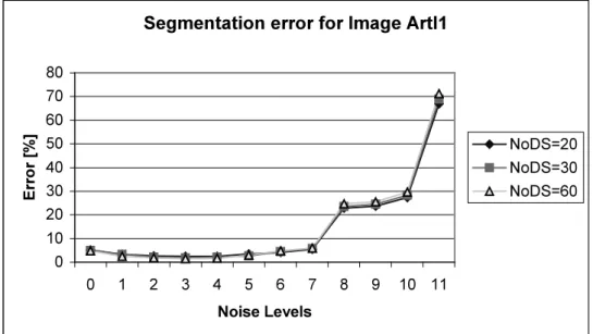
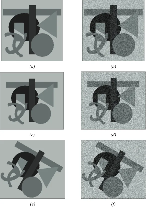
The CNN-MRF model was tested both on artificial and natural images. In the first case the artificially generated pictures consisted of well-defined regions of given number of classes. These original images were loaded with heavy noise and the segmentation algorithm was expected to reconstruct the same homogenous regions as the original image had. In this case comparing the noise-free and the segmented image pixel by pixel we could measure the segmentation error. In case of natural born images the evaluation of the segmentation results is much more difficult. Generally, the comparison is based on hand-made segmentation, or results are evaluated by other subjective means. Only a few cases allow reliable comparisons to ground truth data.

Fig. 4 shows the segmentation results using a noisy input test image (SNR=5dB).

Parameters in the segmentation process are: T_k+1=0.95⋅T_k, α=0.3, and β=10.0. The misclassification error is 1.5%. Using the original MMD algorithm on a CM [36] the error is 1.3 %, and it is 1.0% with the Metropolis algorithm [50,48].

We have checked the segmentation error with respect to the number of iteration steps for different α values. We have found that the process is convergent and settles in about 100 iteration steps. In Fig. 5, the unsupervised segmentation of a SPOT satellite image is shown. Here 4 output classes were defined. Parameters are Tk+1 = 0.95⋅Tk, α=0.3 and β=0.5.

It is important to mention that these segmentation results, and also other results generated with a stochastic iterative process are not always absolutely stable and exactly reproducible. Depending on the speed of convergence, initial temperature, etc.

there can be a few fractions of percentage differences in the outcome of the same experiments.

Input noisy image (SNR=5dB) CNN-MRF Segmented Result Figure 4.

Monogrid segmentation of an artificial test image.

Input SPOT Image CNN-MRF Segmentation

Figure 5.

Satellite Image Segmentation, 4 classes.

3.4 Nonlinear Diffusion for Detail Conservation

In [93] it has been shown that the segmentation error of the CNN-MRF algorithm significantly depends on the type of diffusion used to calculate the expected value and the variance in each pixel position. Nonlinear (or anisotropic) diffusion methods are

much more satisfactory to generate s_s, the average value around pixel s used in Eq.

(14) and Eq. (15), than linear smoothing operators.

While linear smoothing is defined by equation:

) (gradI dt div

dI = , (18)

edge driven diffusion defined by Perona, Malik and Catté [12,67] is given by:

(

)

(g grad G I gradI dt div

dI = o ∗ , (19)

where G is a Gaussian pre-smoothing filter for noise suppression, and

⎟⎟

⎠

⎞

⎜⎜

⎝

⎛−

=

n

K

g exp id , (20)

K>0, n>0, typically n=2. K can control the edge conservation property of the filter.

A simpler equation for nonlinear isotropic diffusion was proposed in [79]:

(

)

dt g

dI = o . (21)

Since in case of both nonlinear solutions g is given by an exponential form the direct implementation of these nonlinear models would require a physically hardly realizable function at each cell. That is why the exponential function is replaced by a linear term detailed in a following section.

3.5 Multigrid Models

Nowadays multiresolution, multiscale, hierarchical approaches are widely applied in the field of image processing. Markov Random Fields are one typical area where the advantages of such techniques seem to be tremendous. A review on this widespreading area can be found in [32]. It is worthy to note that there is a certain confusion in the terminology regarding techniques processing images on more than one representation level. The words like multigrid, multiresolution, multiscale, hierarchical are to be considered generally synonyms, while in some papers they are addressed specially to some well-defined techniques. In this dissertation I usually call the models simply monogrid or multiscale/multigrid depending on whether we apply multiresolution processing or not.

Here are some reasons why multigrid models are usually preferable:

• In a general case many phenomena (e.g. fractal-like signals) have intrinsic multiscale properties so it may have a natural meaning to apply similar operators on different scales.

• In our case we face an optimization problem with possible local minima.

Multiscale optimization can avoid being trapped in local minima. It can also result in faster convergence and become less sensitive to initial configurations.

Generally speaking, the common feature of all multiscale models is the representation of images on several levels with decreasing resolution, while there can be significant differences in the definition of cliques and energy functions in the different approaches (see [32] for details).

The VLSI implementation of the CNN-MRF model with a third order neighborhood- system can be technologically costly, on the other hand, as experienced, our simple cell-array system with first order neighborhood connectivity and with unsupervised pixel-level parameter estimation does not give satisfactory results. What it is expected from multigrid implementations is to reduce the necessary neighborhood connectivity of the monogrid CNN-MRF model at comparable segmentation results and acceptable ratio of the number of operations per iteration.

Multiscale representation can be introduced into a parallel 2D cell-processing framework in two different ways:

1. At lower scale representations rectangular groups of pixels are restricted to have the same value. The size of the image array is constant; these restrictions are responsible to achieve lower resolutions. In this case there is no need for moving or reorganizing the pixel values when changing resolution. However, if we do not want to exceed first order connectivity, only two level image pyramids are feasible this way.

2. The size of the image arrays is changing with resolution. When increasing or decreasing the resolution, pixels should be read out from the 2D array, reorganized and downloaded in a serial process.

These two solutions are equivalent in segmentation, however, they need different computational complexity and memory requirements when implemented in the parallel 2D processor array.

3.6 The CNN-MRF Multiscale Model

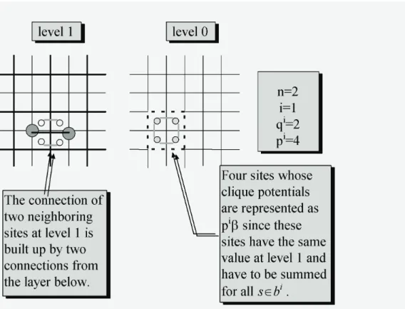
Now, I introduce a multiscale structure for the CNN-MRF model [18]. While the proposed multiscale model is similar to [35], I certainly had to take into consideration the capabilities of the CNN-UM platform where it is supposed to be implemented. In this model we have a top-down strategy from coarser representation of the image to finer scales (in experiments 2x2 sites were used to build up a coarser block, i.e. the re- scale ratio n equals 2). The optimization starts on the coarsest level and the obtained equilibrium state serves as the initial state for the further optimization on the finer layer below. During the optimization process there are no interactions between the scales except for the initial data.

An important feature of this model is the calculation of clique potentials. At a given scale the second part of the energy term (E₂) is calculated through the cliques of the finest scale. While at all levels the cliques of the finest representation are considered for computation, there is a restriction that blocks of n²ⁱ sites must have the same value.

Here n is the re-scale ratio, i is the actual level of representation in the image pyramid.

Cliques, always defined on the finest scale, corresponding to a block at a certain level, can be partitioned into two sets. The first set contains cliques that belong to sites all inside the block, whereas the other set of cliques consists of the ones that connect sites of two neighboring blocks. The energy contribution of the first set is given by pβ in Eq. (22) while Eq. (24) gives the energy of the other set. Clique potentials at a given scale are the sum of these energies measured on the finest resolution.

The following forms represent all energy components at level i similarly to Eq. (9) with the modifications corresponding to the description given above:

σ β μ σ μ

π ω

ω ^{F E F ω p}

E

i si

s i

i

i

b

s s

s s S

s s

i i

i ⎟⎟−

⎠

⎞

⎜⎜

⎝

⎛ −

+

=

=

∑ ∑

∈

∈ 2

2 1

1 2

) ) (

2 ln(

) , ( )

,

( (22)

and

) ( )

2(

i i C i i

i

E

E ω

∑

∈

=

&L

(23) where

⎩⎨

⎧

≠ +

=

= −

=

∑

∈ r s

s r D

s

r r s

i i

if q

if E q

E

Ci β ω ω

ω ω ω β

ω ω

) , (

) , ( )

( . (24)

Explanations to the notations of the above equations:

• ωsimeans the labeling of one block at scale i.

• s∈b_sⁱimeans sites of the finest scale, which build up a block at scale i.

• Cⁱ is one clique, while Cⁱ is the set of all cliques at scale i.

• DCi is the set of those sites which build up clique Cⁱ.

• The number of cliques included in one block at scale i is p=2nⁱ(nⁱ-1), while the number of cliques between two neighboring blocks is q =nⁱ.

Note that these equations apply only for a first order neighborhood-system since our purpose is to reduce the necessary neighborhood connectivity of the monogrid CNN- MRF model.

Fig. 6 represents the two kinds of cliques mentioned, and Fig. 7 illustrates the main steps in the optimization that are:

1. Energy optimization of a layer.

2. Initialization of the next layer from a coarser layer above.

Figure 6.

Multiscale cliques.

Figure 7.

Main steps of multiscale segmentation.

3.7 Experiments with the Multigrid CNN-MRF Model

Besides the model described in the previous section I investigated other multigrid models, e.g. a causal hierarchical model similar to [10]. Here I do not deal with other multigrid algorithms, since the limited set of operations available in our parallel framework did not lead to satisfactory segmentation results with these models.

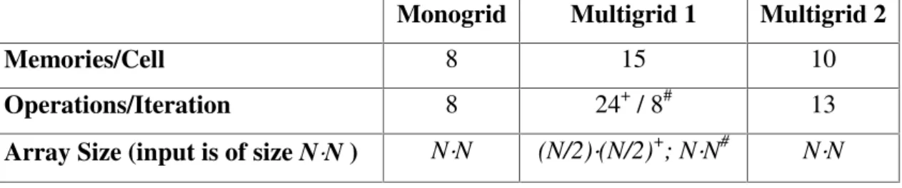
We have found that two implementations of the CNN-MRF multiscale model could work properly in the CNN-UM or in other similar structures. Both of these multiscale implementations need more local memories per cell and functionality than the monogrid version but use only first order neighborhood connectivity.

There are two possible algorithmic implementations of the proposed multiscale model:

1. The first realizes the model just as given by Eq. (22) and Eq. (24).

We start the algorithm at the coarsest scale where the image size is naturally smaller than the input image. Since we work on a chip of fixed size, other parts of the array are not used except for the finest level. Local observations (Eq. (14) and

Eq. (15)) are smoothed then re-scaled and stored for all scales independently.

When the segmented image is stable, then all labels are read out and mapped to a higher resolution by duplicating sites.

2. The second implementation realizes directly the idea that is behind the formulae. In this case we have only the finest scale represented in the cell array and instead of building a coarser (smaller) grid we restrict the values of sites so as to be the same in every block defined on a higher scale. It means that there is no need for the reconfiguration of sites when changing resolution. Initial observations (expected value and variance) are downsampled for lower resolutions and doubletons (Eq. (12)) are computed for all sites of the finest resolution. The crucial point of this implementation is the summation of energy terms over blocks of nⁱxnⁱ pixels at scale i. Since we should not exceed first order neighborhood connectivity only blocks of size 2x2 are appropriate, larger areas are not adequate for collecting and summing up clique potentials. Thus only two level pyramids are supported by this construction. The generation of random labels is clear: since they are generated by offset of the first iteration, spatial restrictions apply only in the first random step.

Since both techniques are based on the same theory, very similar segmentation results are expected, however, they have different complexity and different computation time. In our experiments both models were optimized with the MMD technique with various ad hoc parameters.