HISTOGRAM BASED SEGMENTATION OF SHADOWED LEAF IMAGES 1

DOI: 10.1556/606.2018.13.1.2 Vol. 13, No. 1, pp. 21–32 (2018) www.akademiai.com

HISTOGRAM BASED SEGMENTATION OF SHADOWED LEAF IMAGES

1 Tamás STORCZ, ² Zsolt ERCSEY, ³ Géza VÁRADY

1,2 Department of Systems and Software Technologies, Faculty of Engineering and Information Technology, University of Pécs, Boszorkány u. 2, H-7624 Pécs, Hungary

e-mail: ¹storcz.tamas@mik.pte.hu, ²ercsey@mik.pte.hu

3 Department of Information Technology, Faculty of Engineering and Information Technology University of Pécs, Boszorkány u. 2, H-7624 Pécs, Hungary, e-mail: ³varady.geza@mik.pte.hu

Received 27 February 2017; accepted 1 August 2017

Abstract: This paper corresponds to the solution of some problems realized during ragweed identification experiments, namely the samples collected on the field by botanical experts did not match the initial conditions expected. Reflections and shadows appeared on the image, which made the segmentation more difficult, therefore also the classification was not efficient in previous study. In this work, unlike those solutions, which try to remove the shadow by restoring the illumination of image parts, the focus is on separating leaf and background points based on chromatic information, basically by examining the histograms of the full image and the border.

This proposed solution filters these noises in the subspaces of hue, saturation and value space and their combination. It also describes a qualitative technique to select the appropriate values from the filtered outputs. With this method, the results of segmentation improved a lot.

Keywords: Ragweed, Leaf, Shadow, Segmentation, Histogram statistics

1. Introduction

Supervision of vegetation gain importance in rural and according to nowadays trends also in urban environments [1]. For economical and health care reasons, the main task of the research group for ragweed exemption workgroup is the identification of ragweed (Ambrosia Artemisiifolia L.) from a short distance by optical observation.

Besides the work described by Schiffer et al. [2] and Jacskár et al. [3], other ideas are also investigated. As the first step of a complex solution, it has to be decided if the ragweed can be identified by its leaves’ images or not. To prove this assumption, an image classifier system was proposed (see Storcz and Ercsey [4. p. 22], [4, p. 26]),

containing a statistical moment invariant [5], [6] based feature extraction and perceptron based multilayer neural work [7]. With this, the possibilities of plant species classification by their full leaves, observed from above were examined. The initial conditions declared for the samples are: full, flat leaf, observation direction is perpendicular to the plane of leaf, the background is non-reflective homogenously colored. To refine the results, extension of the sample space became necessary.

Therefore botanical experts were involved, to create real field samples under natural circumstances (light direction, intensity, live plants, immediate processing). The subject was the ragweed, and the most similar species indigenous in Hungary.

The performance of the classifier system was measured with the following inputs:

• geometrical shapes - binary images created from 2D shapes by applying geometrical transformation (scale, rotation, translation);

• supervised leaf samples - color and binary samples from other experiment [7], [8], [9] do not contain ragweed and are referred as contrary samples. Those which are collected in the scope of the main task, with subject of ragweed are referred as pro samples and all conform the initial conditions;

• unsupervised leaf samples - real field samples, created by botanical experts under natural conditions. Also referred as contrary samples where supervised sampling is when a supervisor helps sample collectors to keep sampling restrictions, hence providing expected sample quality.

In the first two sample spaces, the performance was above 98%, but in the third, the identification ability of ragweed leaf dropped back to 71%. The performance fall-back could have been caused by the low classification capability of the ragweed leaf, but it was not obvious. Therefore, to understand the reason of the fall-back better, a revision in each sample space was carried out. As the result of the revision the followings have been established. The field samples only partially conformed the necessary initial conditions, therefore the applied histogram based segmentation algorithm made mistakes in separating leaf and background pixels. The incorrect shape segmentation resulted incorrect classification.

Human confirmation based segmentation verification showed 100.0%, 99.8% and 65.5% segmentation accuracy, according to the previous order (geometrical, supervised, and unsupervised). The final value shows that the pre-processor and segmentation algorithm requires enhancement.

The analysis of field samples pinned out the following important problems:

• Shadowed regions appeared, dropped by the leaf parts, which were out of its main plane. The reason behind is breaching the ‘perpendicular observation of flat leaf’ condition;

• The background on the sample images showed different inhomogeneity, even if it looked homogeneous. Due to the reflective properties of the material and the varying intensity and direction of the natural illumination the camera recorded extra reflections, which were not realized at the time of sampling. This ruins the

‘homogenous, non-reflective background’ condition;

• The intensive, non–perpendicular illumination and the uneven surface, presented in the first point, resulted under-saturated (closed to black and white) areas, independently from the chromatic properties of the surface.

These disturbing factors significantly influenced the efficiency of the histogram based image segmentation, which obviously reduced the accuracy of the final result.

The problems presented above, and the absence of color restrictions together resulted that there is no uniform method for statistical segmentation of the extended sample space.

Unfortunately the repetition of sampling is not possible because of the expenses of the expert participation, and of the delay for almost a year by the growing period of the subject plant species. To continue the experiments, a complex pre-processing and segmentation method is needed, which can be applied to filter the noises discussed earlier, and its development and operation can be quick enough not to delay the main tasks.

2. Related work

There are references widely available about removing shadows from still images and video sequences, because this is a cardinal question of image content analysis and machine vision. The basic problem is that in image interpretation the shadowed areas could appear as individual surface components. Generally, the solutions consist of the following two steps. First, the identification of shadowed areas then decreases the effect of shadowing by artificially increasing the illumination of the affected regions.

Deb and Suny [10] specifies a binary shadow mask from the full image and the general intensity of a 3x3 sliding window on the result of an RGB - YCrCb conversion [11]. The pixel intensity ratio on the two sides of a shadow edge can be used to reconstruct the shadow-free image. The Cr and Cb subspaces can be used for chromatic correction along the eliminated shadow edges. Fredenbach and Finlayson [12] also use the same ratio. But instead of thresholding from local and global intensities, they compare the raw and illumination invariant images to mark shadow edges. From these, they form closed shapes. Along the borders of these regions, from the intensity of shadowed and non-shadowed pixels, they compute constant illumination differences for each color channels. Finally these constants are used to increase illumination of shadowed areas. Xu et al. [13] extend the shadow model from above by searching for two types of shadow edges. First to find partially shadowed images, perform edge detection in the low-pass filtered gradient domain. Then to locate fully shadowed edges, perform other edge detection in the illumination invariant image. This is computed as a difference of the raw image and the hue subspace of the Hue, Saturation and Value domain (HSV space) [11]. Shadow removal is also evaluated along the shadow edges by setting gradients to zero. The inverse approximation problem was resolved by solving the Poisson-equation.

P. Sharma and R. Sharma [14] used illumination invariant, illumination invariant and neighboring similarity features for shadow edge classification of patch borders.

Barnard and Finlayson [15] constructed a similar, but simplified method. They constructed a Look-Up-Table (LUT) for the intensity rates of pixels appeared on the

sides of the patch borders on a pre-segmented image. Based on this LUT, a decision can be made about if the edge can be a shadow edge or not. The authors use the same intensity rate to correct the illumination of the shadowed regions.

Levine and Bhattacharyya [16] tend to enhance the previous method. As pre- processing steps, the applied luminance based multi scale retinex, and mean shift color image segmentation. The basic idea of their improvement is that the main weakness of thresholding methods is to select a good threshold value. Therefore these methods are replaced by machine learning components. In the method, first, a Support Vector Machine (SVM) decides if the edge is well saturated or not. In both cases, other SVM (one for each) estimates the probability of under illumination (shadow). Upon the shadow data of borders, the fourth SVM decides whether a region is shadowed or not. If yes, the new intensity is derived from the intensity values of surrounding areas.

Khan et al. [17] use two convolutional neural networks to identify shadow regions.

Nowadays, these structures came to the interest of many researches. Their forward connected networks use 7 convolutional layers, alternating convolution and max- pooling. One was taught to identify the borders and one to identify the interior of the shadowed regions. The results of the Convolutional Networks were fed to a conditional random field model to integrate them into continuous, closed regions. After the creation of a shadow mask, any of previous methods could be used to adjust illumination.

Some shadow detection and shadow removal methods were studied by Rashmi et al.

[18]. During the simple comparison, they found that the color based method and Otsu’s thresholding are the most efficient methods for shadow detection after its removal of an image. The main disadvantages of the reviewed methods are that both listed methods consider shadows to be removed irrelevant to their nature. Song et al. [19] considered shadows in high resolution satellite images, proposing morphological filtering for shadow detection and an example-based learning method for shadow reconstruction.

This recent work focused to attenuate the problems caused by the loss of radiometric information in shadowed areas. Salih et al. [20] also worked on very high resolution satellite images. The first tested novel method detected shadows by the ratio between near infrared and visible bands on a pixel by pixel basis. The other technique they tested was the kernel graph cut algorithm. As a conclusion they are conceived that there is no general solution. The appropriate method depended on the characteristics of the source image. Unfortunately the method to obtain the boundary conditions from processed images described by Jancskár [21] cannot be used sufficiently for shadow detection.

The main disadvantage of the solutions above is not handling the over- and under illuminated regions properly. Furthermore, they require high computational power.

Implementation difficulties can also occur, because the required parameters, kernel functions, teacher and validator samples are not available. Thus, the main goal is to create a simple pre-processor method with noise filtering and segmentation, which can be easily implemented, does not contain unknown parameters, and can prepare any field samples for the further evaluation processes with an acceptable efficiency and speed. To achieve this chromaticity an intensity information based methods reviewed by Chondagar et al. [22] is adopted. Neither the types of shadows they defined nor the over illuminated areas should matter for the proposed method. This work was partially inspired by publication of Digarse at al. [23], in which the color features were used to assist shadow recognition directly, and to refine the illumination map. In other words,

pixel intensities were compared with respect to chromaticity values. They used the correlation of local luminance contrast and average local luminance.

3. Histogram based logical segmentation

The histogram based segmentation method (1) separates the pixels of subject from the background based on number of occurrences of pixel intensities. The method is general, because only the intensity histogram and not the location of pixels are taken into consideration. The logical attribute refers to the logical output

( ) ( ) ( ) ^{( )}

( ) ^{X Y}

y x I c

x y cI x y Ic x y I M

c hist

y x I c

, , ,

1 and

0

, 1

, where ,

,

,

°¯ ∈

°®

=­

=¦ ¦

≠

= , (1)

where I(x,y) is color intensity at row y column x; c is the examined color; Ic(x,y) is the logical intensity and histl is the logical histogram of color c, MX,Y is the image with size of X columns and Y rows.

At the beginning of the segmentation there is no data about the image part size occupied by the subject, nor the logical value, which represents it. Therefore, it is obvious that only the intensity histogram is not enough. In both Fig. 1a and Fig. 1b white color is dominant, however on the earlier white represents the subject, but on the other it represents the background.

a) Great white subject b) Great white background Fig. 1. Black & white source image types

To make the method of logical segmentation (1) applicable, the generality is slightly decreased. Another histogram form pixels of a k pixel wide border of the image (2) is computed. With these two histograms and the assumption that the subject on the image takes more space closer to the center than the sides, the colors of the subject can be determined. All others represent the background

( ) ( ) ( ) ( ) ( )

( )

( )

( )

( )

, ,

, ,

1 1 1

0

1 1 1

0

1 1 1

0 1

0

1 1

0

¦ ¸¸

¹

·

¨¨

©

§ ¦ + ¦

¦ ¸¸+

¹

·

¨¨

©

§ ¦ + ¦

+

¦ ¸¸

¹

·

¨¨

©

§ ¦ + ¦

¦ ¸¸+

¹

·

¨¨

©

§ ¦ + ¦

=

−

−

=

−

−

=

−

=

−

−

=

−

−

=

−

=

−

−

=

−

−

=

−

=

−

=

−

−

=

−

=

k Y

k y

X k X

x c

k

x c

k X

k x

Y k Y

y c

k

y c

X k X x

Y k Y

y c

k y c k

x

Y k Y

y c

k

y c

frm

y x I y

x I y

x I y

x I

y x I y

x I y

x I y

x I c

hist

(2)

where X, Y are image (width and height); k is the frame width; histfrm is the frame histogram.

According to (3), the most frequent color in the frame histogram refers to the background, the other color is the subject,

( ) ( )

,

, max

where ,

_ fore back

frm frm

back

C C

hist c

hist c

C

=

=

=

(3)

where Cback is background; Cfore is the subject color, C is the set of all colors.

This solution assumes logical inputs (2 possible values) but not sensitive to the inverse representation.

4. Enhanced methods

Bicolor images

From the point of enhancement of the method, the simplest case is the segmentation of bicolor images. By definition, these images contain only 2 colors, but unlike logical inputs, these 2 values could be any of a wider interval. To handle them, the histogram is extended with all values of the source domain interval, and rebuilds the histograms of (1) and (2). The difference of logical and bicolor histogram is visible in Fig. 2a and Fig. 2b.

a) Logical histogram b) Bicolor histogram c) Histogram of 32 colors with 2 dominant Fig. 2. Histogram types

Data of new border and full histograms are evaluated according to (4). With this, the main colors of the subject and the background can be selected. The most frequent color in the frame histogram refers to the background, the other most frequent color is the subject,

( ) ( )

( )

( )

( )

where ,

,

, max

where ,

rem rem

fore

C img c rem

frm frm

back

hist c

hist c

C

c hist hist

hist c

hist c

C

back

=

=

=

=

=

≠ (4)

2 fore back threshold

C

C C +

= , (5)

where histimg is the histogram of the full image.

An averaging (5) is applied to specify a threshold value. The application of this threshold separates the main colors by bisection of the intermediate region. With this, the histogram based segmentation method is already applicable for intensity images, which contain all possible colors, but the colors of the homogenous subject and background are prevailing. A histogram of this sort is presented in Fig. 2c.

Processing of images mentioned above comes to the front if a noise filtering (for example blurring) is applied on black and white (logical) images. Depending on the filter settings, this results in a small amount of intermediate colors between the dominants. This is applicable because carefully set blurring does not change the position of edge gradients and their intensity also stay above a well selected threshold.

This type of image also can be created by grayscale sampling of the scene, which fully satisfies all our initial conditions of sampling.

Grayscale images

On real field samples, like on bicolor images, pixel intensity values are in a specific interval defined by the sampling device. However, the constraint of two dominant colors is breached by the illumination properties, inaccuracy of sampling device and the natural chromatic inhomogeneity of the subject’s material. When trying to insist on the initial condition of inhomogeneity, the deviation would not be significant. Therefore, in the histogram, the single column of the dominant colors would transform into a bell curve.

Fig. 3 shows an example of appearance of a bell curve in a histogram. Fig. 3a shows the original grayscale image. Fig. 3c is the smoothed full histogram. In this two peaks can now be identified. One peak is the subject and the other is the background. The selection is supported by Fig. 3d, the smoothed histogram of the border. According to (4) its only peak refers to the peak of background color in the full histogram. The other peak in Fig. 3c is the subject color. To separate these colors, the intermediate interval is split in its middle as (5) specifies, or can threshold at the position of minimum value.

Fig. 3b shows the result of logical separation based on the method proposed above.

Color images

According to the parameters of the non-professional, mobile devices available for field sample creation, it could be expected or even more required to use a camera, which is able to record in RGB format [11]. Therefore, the focus is on this type of samples.

The processing of color images by color channels is not ideal, because there are no initial constraints for the colors. This may also mean that the homogeneity does exist in the RGB image, but the difference between the subject and the background is distributed between the color channels. As a result, the separation is much harder.

Based on the issues above, to summarize the chromatic difference and increase the ability of processing the color channel values are combined with intensity values.

Indeed, the color image is converted into grayscale as (6) explains. After this conversion, the sample images could be processed as described in subsection of Grayscale images.

Blue Green

Red

gs C C C

I =0.2126⋅ +0.7152⋅ +0.0722⋅ , (6)

where CRed, C_Green, CBlue are intensities of red, green and blue color channels; Igs is the grayscale intensity.

a) Grayscale image b) Binary image

c) Smoothed full histogram d) Smoothed border histogram Fig. 3. Histogram based on segmentation steps

Shadowed images

The surface irregularities of the subject leaf result in shadow drops. These shadowed areas may appear on the background, and also on the leaf itself. This can heavily decrease the segmentation accuracy, because the shadowed regions could be identified as separate surface elements. This is presented in Fig. 4, where Fig. 4a is the original intensity image; Fig. 4b is the smoothed histogram. Fig. 4c is the segmentation result, which contains some parts of the leaf and the shadowed background. To successfully process this kind of images, they are transformed them into an illumination invariant space. To achieve this, the hue subspace of the HSV space [11] is selected. By this transformation the influence of the illumination changes are eliminated. The result is presented in Fig. 5 in the order as Fig. 4 was described.

Under-saturated image parts

In some of the samples created in unsupervised manner, because of the chromatic properties of the background and illumination/shadowing errors, light- and/or dark grey

pixels appeared. The interpretation of these pixels was unsuccessful in the intensity, and also in color temperature space as shown in Fig. 6a, Fig. 6b, Fig. 6d, Fig. 6e.

a) Intensity image b) Intensity histogram c) Intensity mask Fig. 4. Intensity based segmentation

a) Hue image b) Hue histogram c) Hue binary image Fig. 5. Hue based segmentation

a) Intensity image b) Hue image c) Enhanced hue image

d) Intensity mask e) Hue mask f) Enhanced hue mask Fig. 6. Segmentation results from different sources

To handle this type of pixel noise, a white and a black group are created from them, by thresholding their intensity at 50%. Then they are integrated into the linearized color ring. First the color temperature values are re-indexed. The RGB-HSV transformation

linearized the color circle to the [0..1] interval. It is re-quantized to ]1..63[, then the red color is moved from both sides to the end (63). Finally, the white and black groups are added to the sides of the interval, into position 0 and 64, regardless of the color temperature values. The result of segmentation based on re-indexed and extended linear color temperature values is shown in Fig. 6c and Fig. 6f.

Selection of the method to apply

Unfortunately none of the methods explained above is suitable to completely solve all of the described challenges. The best result can be achieved by applying the most appropriate method for the actual image. To make this selection automatic, a fuzzy membership function is declared, based on maximum points of all full and border histograms. The decision selected a membership function with less transition or if it was the same for more, the one with wider averaged transition interval. The defuzzification was made at interval bisection of interval minimum point selection.

5. Results

The segmentation of geometric shapes (3000 pcs) and samples in supervised manner (2466 pcs) were over 99% with both the initial and the proposed algorithm. The segmentation accuracies of leaf samples are summarized in Table I. The accuracy was measured by confirmation or rejection by a human controller.

Table I

Segmentation accuracy of methods

Number of

samples

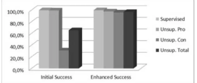
Initial Success Enhanced Success Count Rate Count Rate Supervised 2466 2462 99.8% 2464 99.9%

Unsupervised Pro 394 392 99.5% 385 97.7%

Unsupervised Con 389 121 31.1% 374 96.1%

Unsupervised

Total 783 513 65.5% 759 96.9%

The segmentation accuracy of 394 pcs ragweed samples was dropped back a little from 99.5% to 97.7%. Instead of the initial 2 errors another 9 arose. That was because of the negligible size of subject leaves on the incorrect images. From the total 170 K pixels of the images leaves consist of only 1500 pixels, which is less than 1% of the image size. This size is similar to a size of different noise types, therefore leaves were also identified as noise.

From the 389 pcs unsupervised samples, created by botanical experts on the field, the initial algorithm could properly segment only 121 pcs, which is 31.1%. With the proposed algorithm that was raised to 374 pcs, which is 91.1%.

Fig. 7 shows that from the summarized 783 pcs of pro and contra unsupervised samples the initial algorithm could properly segment 65.5%. The proposed algorithm could increase this to 96.9%.

The available 3249 pcs of samples were segmented in 1313 secs, by the C#.Net implementation of the initial algorithm. The GNU Octave 4.0.0x64 implementation of the enhanced algorithm required only 851 secs. Both included load and save disk operations, were executed on a desktop computer equipped with Intel Core I5@3.1 GHz processor and 8 GB RAM. Processor or GPU parallelization were not used in any of the implementations.

Fig. 7. Segmentation accuracy

6. Conclusion

In this paper methods were presented to remove shadows by separating leaf and background points based on chromatic information, by examining the histograms of the full image and the border and filtering noises in the subspaces of HSV space and their combination. A fuzzy based technique to select the appropriate method was given also.

The studies shows that the proposed solution provided segmentation accuracy well enough on samples, which only partially satisfy the initial conditions. The method increased the segmentation accuracy from 65.5% to 96.9%. With this the classification can be repeated, the ragweed identification research can be continued.

However, it is also visible that general histogram based segmentation is not suitable for general separation of subjects and backgrounds of images bothered by shadows and pixel noise.

Acknowledgement

The present scientific contribution is dedicated to the 650th anniversary of the foundation of the University of Pécs, Hungary.

References

[1] Szkordilisz F. Mitigation of urban heat island by green spaces, Pollack Periodica, Vol. 9, No. 1, 2014, pp. 91−100.

[2] Schiffer A., Sari Z., Müller P., Jancskar I., Varady G., Ercsey Zs. Ragweed detection based on SURF features, Technical Gazette, Vol. 24. No. 5, 2017, pp. 1519௅1524.

[3] Jancskar I., Sari Z., Schiffer A., Várady G. Phase plane tuning of fuzzy controller for 1 DoF helicopter model, Pollack Periodica, Vol. 10, No. 2, 2015, pp. 3௅15.

[4] Storcz T., Ercsey Zs. Ragweed recognition: statistical feature extraction and CNN classification, (in Hungarian) Pollack Press, 2015.

[5] Hu M. K. Visual pattern recognition by moment invariants, IRE Transactions on Information Theory, Vol. 8, No. 2, 1962, pp. 179−187.

[6] Sabhara R. K., Lee C. P., Lim K. M. Comparative study of Hu and Zernike moments on object recognition, Smart Computing Review, Vol. 3, No. 3. 2013, pp. 172−177.

[7] Mitchell T. M. Machine learning, McGraw-Hill, 1997.

[8] Wu S. G., Bao F. S., Xu E. Y., Wang Y. X., Chang Y. F., Xiang Q. L. A leaf recognition algorithm for plant classification using probabilistic neural network, 7th IEEE International Symposium on Signal Processing and Information Technology, Cairo, Egypt, 15-18 December 2007, pp. 11−16.

[9] Tree Leaf Database MEW2010, Department of Image Processing, Institute of Information Theory and Automation, Academy of the Sciences of Czech Republic, http://zoi.utia.

cas.cz/tree_leaves (last visited 27 December 2016).

[10] Deb K., Suny A. H. Shadow detection and removal based on YCrCb color space, Smart Computing Review, Vol. 4, No. 1, 2014, pp. 23−33.

[11] Noor A. I., Mokhtar M. H., Rafiqul Z. K., Pramod K. M. Understanding color models, A Review, ARPN Journal of Science and Technology, Vol. 2, No. 3 2012 pp. 256−275.

[12] Fredembach C., Finlayson G. Simple shadow removal, Proc. of the 18th International Conference on Pattern Recognition, Hong-Kong, China, 20-24 August 2006, Vol. 1, pp. 832௅835.

[13] Xu L., Qi F., Jiang R. Shadow removal from a single image, Proc. of 6th International Conference on Intelligent System Design and Applications, Washington DC, USA, 16-18 October 2006, Vol. 2. pp. 1049−1054.

[14] Sharma P., Sharma R. Shadow detection and its removal from images using strong edge detection method, Journal of Electronics and Communication Engineering, Vol. 10, No. 4, Ver. II, 2015. pp. 72−75.

[15] Barnard K., Finlayson G. D. Shadow identification using color ratios, Proc. of 8th Color Imaging Conference, Scottsdale, Arizona, USA, 7-10 November 2000, pp. 97−101.

[16] Levine M. D., Bhattacharyya J. Removing shadows, Pattern Recognition Letters, Vol. 26, No. 3, 2005. pp. 251−265.

[17] Khan S. H., Bennamoun M., Sohel F., Togneri R. Automatic feature learning for robust shadow detection, Proc. of IEEE Conference on Computer Vision & Pattern Recognition, Columbus, Ohio, USA, 23-28 June 2014, pp. 4321−4328.

[18] Rashmi V., Srinivas R. V., Srinivas K. Comparative analysis of shadow detection and removal methods on an image, Special Issue International Journal of Computer Science and Information Security, Vol. 14, 2016, pp. 152−156.

[19] Song S., Huang B., Zhang K. Shadow detection and reconstruction in high-resolution satellite images via morphological filtering and example-based learning, IEEE Transactions on Geoscience and Remote Sensing, Vol. 52, No. 5, 2014, pp. 2545−2554.

[20] Salih N. M., Kadhim M., Mourshed M., Bray M. T. Shadow detection from very high resolution satellite image using grab-cut segmentation and ratio-band algorithms, The International Archives of the Photogrammetry, Remote Sensing and Spatial Information Sciences, Vol. XL, No. 3/W2, 2015, pp. 95−101.

[21] Jancskar I. IR-image based inverse radiative heat transfer problem, Pollack Periodica, Vol. 8, No. 1, 2013, pp. 75−87.

[22] Chondagar V., Pnadya H., Pnachal M., Patel R., Sevak D., Jani K. A review: shadow detection and removal, International Journal of Computer Science and Information Technologies, Vol. 6, No. 6, 2015, pp. 5536−5541.

[23] Digarse D., Chauhan K. Shadow detection by local color constancy, International Journal of Computer Applications, Vol. 124, No. 14, 2015, pp. 36−41.