2013 ZoltanKato FromRegionstoShapes:TheExtractionandAlignmentofVisualObjects H A S D D D

D ISSERTATION FOR THE D OCTORAL D EGREE OF THE

H UNGARIAN A CADEMY OF S CIENCES

From Regions to Shapes:

The Extraction and Alignment of Visual Objects

Zoltan Kato

Department of Image Processing and Computer Graphics, Institute of Informatics,

University of Szeged, Hungary

2013

I gratefully acknowledge the contributions of my MSc and PhD students from University of Szeged Hungary: Csaba Domokos, P´eter Horv´ath, Zsolt S´anta, Csaba Moln´ar, J´ozsef N´emeth; as well as Guo Qiang Song from National University of Singapore. My colleagues at various institu- tions also provided valuable contributions: Josiane Zerubia and Marc Berthod from INRIA Sophia Antipolis, France; Ian Jermyn from Department of Mathematical Sciences, Durham University, UK;

Ting Chuen Pong and John Chung Mong Lee from Computer Science Department of the Hong Kong University of Science & Technology, Hong Kong; Attila Tan´acs from University of Szeged, Hungary;

Joseph Francos from Ben Gurion University of the Negev, Israel; Jhimli Mitra, Soumya Ghose, and Fabrice Meriaudeau from Le2i-UMR CNRS 6306, Universit´e de Bourgogne, France; Csaba Benedek and Tam´as Szir´anyi from Distributed Events Analysis Research Laboratory of the Computer and Automation Institute of Hungarian Academy of Sciences; Natasa Sladoje from Faculty of Technical Sciences of the University of Novi Sad, Serbia; and Joakim Lindblad from Centre for Image Analysis, Uppsala University, Sweden.

The SPOT satellite images were provided by the French Space Agency (CNES). Lipid droplet mi- croscopy images were obtained from L´aszl´o V´ıgh and Zsolt T ¨or¨ok from Biological Research Centre, Szeged, Hungary; other microscopy images were provided by P´eter Horv´ath from Light Microscopy Centre, ETH Zurich, Switzerland. The fractured bone CT images were obtained from the University of Szeged, Department of Trauma Surgery and were used with permission of Prof. Endre Varga, MD.

Pelvic CT studies and hip prosthesis Xray images were provided by Endre Szab´o, ´Ad´am Per´enyi, Agnes S´ellei and Andr´as Palk´o from the Radiology Department of the University of Szeged. Lung´ CT images and thoracic CT studies were provided by L´aszl´o Papp from Mediso Ltd., Hungary.

Contents Contents Contents Contents Contents Contents Contents Contents Contents Contents Contents Contents Contents Contents Contents Contents Contents Contents Contents Contents Contents

Contents i

Figures vii

Tables xiii

Introduction 1

Extraction of coherent image regions . . . 2

Alignment of visual objects . . . 3

1 Markovian segmentation models 7 1.1 Introduction . . . 8

1.1.1 Markovian approach . . . 9

1.2 Hierarchical MRF models and multi-temperature annealing . . . 10

1.2.1 Multiscale and hierarchical model . . . 10

1.2.2 Multi-temperature annealing . . . 14

1.3 Parameter estimation . . . 17

1.4 Application in remote sensing . . . 20

2 Complex features and parameter estimation 31 2.1 Introduction . . . 32

2.2 Unsupervised segmentation of color textured images . . . 32

2.3 Segmentation of color images via reversible jump MCMC sampling . . . . 36

2.4 Multilayer MRF modelization . . . 41

2.4.1 Application to motion segmentation and change detection . . . 43

3 The ’gas of cicrcles’ MRF model 47

3.1 Introduction . . . 48

3.2 Higher order active contours . . . 49

3.3 The ‘gas of circles’ HOAC model . . . 50

3.3.1 Stability analysis . . . 50

3.3.1.1 Parameter constraints . . . 52

3.3.2 Geometric experiments . . . 53

3.4 Phase field model . . . 55

3.5 Equivalence of the HOAC, phase field, and MRF models . . . 57

3.6 Discretization . . . 58

3.6.1 Quantization of the functionφ . . . 58

3.6.2 Discretization of the domainD . . . 59

3.6.3 Discretization of the energy functional . . . 60

3.6.3.1 Relationship between the parameters of the contour and field energies . . . 62

3.6.3.2 Parameters of the discrete energy functional . . . 62

3.7 Markovian interpretation . . . 62

3.7.1 Singleton potential . . . 64

3.7.2 Doubleton potential . . . 65

3.7.3 Long range potential . . . 66

3.8 The ’gas of circles’ MRF model . . . 66

3.8.1 Experiments . . . 67

3.9 Application in remote sensing . . . 70

4 The multi-layer ’gas of circles’ model 77 4.1 Introduction . . . 78

4.2 Layered representation of overlapping near-circular shapes . . . 78

4.2.1 Functional derivative of the layered energy . . . 80

4.3 The multi-layer MRF ‘gas of circles’ model . . . 80

4.3.1 Energy of two interacting circles . . . 81

4.3.1.1 Different layers . . . 82

4.3.1.2 Same layer . . . 82

Contents iii

4.3.2 Experimental results . . . 83

4.3.2.1 Data likelihood . . . 83

4.3.2.2 Simulation results with the multi-layer MRF GOC model 84 4.3.2.3 Quantitative evaluation on synthetic images . . . 86

4.4 Application in biomedical imaging . . . 86

4.4.1 Performance of the phase field model . . . 86

4.4.2 Results with the MRF model . . . 87

5 Linear registration of 2D and 3D objects 91 5.1 Introduction . . . 92

5.2 Problem statement . . . 93

5.3 Solution via a nonlinear system of equations . . . 94

5.3.1 Registration of 3D objects . . . 97

5.4 Affine puzzle . . . 99

5.4.1 Realigning object parts . . . 99

5.5 Solution via a linear system of equations . . . 101

5.5.1 Construction of covariant functions . . . 102

5.5.2 Linear estimation of affine parameters . . . 103

5.5.3 Choosing the integration domain . . . 104

5.6 Discussion . . . 108

5.7 Medical applications . . . 109

5.7.1 Fusion of hip prosthesis X-ray images . . . 109

5.7.2 Registration of pelvic and thoracic CT volumes . . . 111

5.7.3 Bone fracture reduction . . . 111

6 Nonlinear alignment of 2D shapes 115 6.1 Introduction . . . 116

6.1.1 State of the art . . . 116

6.2 Registration framework . . . 118

6.2.1 Construction of the system of equations . . . 120

6.2.2 Discussion . . . 120

6.2.2.1 Relation to moment-based approaches . . . 120

6.2.2.2 Invariance vs. covariance . . . 121

6.2.2.3 Registration vs. matching . . . 121

6.3 Choice ofωfunctions . . . 122

6.3.1 Normalization . . . 122

6.3.2 Computational efficiency . . . 123

6.3.3 Solution and complexity . . . 125

6.4 Modeling deformation fields . . . 125

6.4.1 Planar homography . . . 126

6.4.2 Thin plate spline . . . 127

6.5 Experimental results . . . 127

6.5.1 Comparison of variousωfunctions . . . 128

6.5.2 Quantitative evaluation on synthetic data . . . 130

6.5.2.1 Robustness . . . 131

6.6 Applications . . . 132

6.6.1 Matching traffic signs . . . 132

6.6.2 Aligning hip prosthesis X-ray images . . . 133

6.6.2.1 Comparison with correspondence-based homography es- timation . . . 133

6.6.3 Matching handwritten characters . . . 134

6.6.4 Fusion of MRI and TRUS prostate images . . . 134

6.6.5 Elastic registration of 3D lung CT volumes . . . 135

6.6.6 Industrial inspection . . . 136

Conclusion 143 Summary of new scientific results . . . 144

A Proof of theorems 149 A.1 Proof of the multi-temperature annealing theorem . . . 150

A.1.1 Notations . . . 150

A.1.2 Proof of the theorem . . . 151

A.2 Proof of Theorem 5.3.1 . . . 160

A.3 Proof of Theorem 6.3.1 . . . 161

Contents v

Author’s publications 165

Bibliography 171

Figures Figures Figures Figures Figures Figures Figures Figures Figures Figures Figures Figures Figures Figures Figures Figures Figures Figures Figures Figures Figures

Chapter 1. 7

1.1 First order neighborhood system with corresponding cliques. . . 9

1.2 The isomorphismΦⁱbetweenBⁱ andSⁱ. . . 11

1.3 The neighborhood systemG¯and the cliquesC¯1,C¯2andC¯3. . . 11

1.4 Results obtained by the Gibbs Sampler [97] on a noisy synthetic image (128×128, SNR = 10dB) with 16classes [14, 20–24]. In the table, we show for each model the number of iterations, the CPU time, the error rate of the segmentation (=the number of misclassified pixels) and the inter- and intra-clique potentialsβandγ. . . 13

1.5 Results obtained by ICM [64] on a (256×256) SPOT image with4classes [14, 20–24]. . . 13

1.6 Energy decrease and segmentation results of the Gibbs sampler on a syn- thetic image with the inhomogeneous and MTA schedules. In both cases, the parameters were strictly the same, the only difference is the applied sched- ule. We also show the global energy plot (computed at a fixed temperature on the finest level) versus the number of iterations. Note that both schedules reach practically the same minimum (53415.4 for the inhomogeneous and 53421.4 for the MTA), however the inhomogeneous schedule requires238 iterations (796.8sec. CPU time) while the MTA schedule requires only100 iterations (340.6sec. CPU time) for the convergence [20, 24]. . . 17

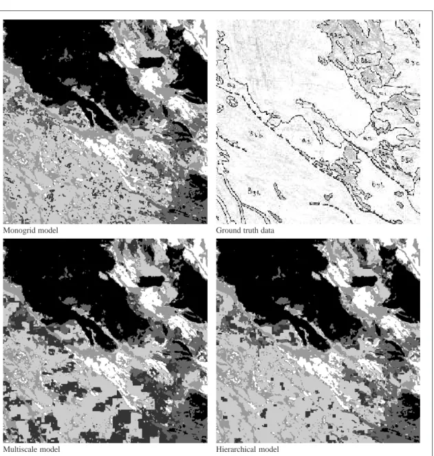
1.7 Supervised and unsupervised segmentation results and misclassification rate with the Gibbs Sampler. We also compare the parameters obtained by the unsupervised algorithm to the ones used for the supervised segmentation [25, 36–38]. . . 21

1.8 Original SPOT image “assalmer” with 6 classes. . . 22

1.9 Ground truth data. . . 23

1.10 Results of the ICM algorithm. Comparison with ground truth data. . . 24

1.11 Results of the Gibbs Sampler. Comparison with ground truth data. . . 25

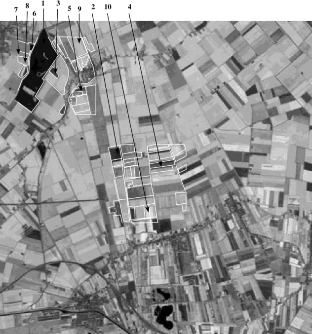
1.12 Training areas on the “holland” image. . . 26

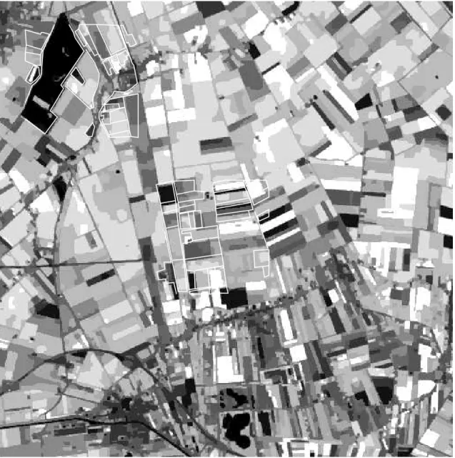
1.13 Supervised segmentation result with10classes (Gibbs Sampler). . . 27

1.14 Unsupervised segmentation result with10classes (Gibbs Sampler). . . 28

Chapter 2. 31 2.1 Unsupervised segmentation results on color textured images, each with 5

classes [28]. . . 35

2.2 ψ is a diffeomorphism which transforms back and forth between parameter subspaces of different dimensionality [15, 16]. Dimension matching can be implemented by generating a random vectoru such that the dimensions of (X, u)andX^′ are equal. . . 37

2.3 Segmentation of image rose41 and the estimated Gaussian mixture [15, 16]. 38 2.4 Benchmark results on images from the Berkeley Segmentation Dataset [16] 39 2.5 Precision-recall curve, F-measure and CPU time comparison for JSEG and RJMCMC [16]. . . 40

2.6 Multi-layer MRF model [27, 29]. . . 40

2.7 Three-layer MRF model for change detection [2]. . . 40

2.8 Segmentation results [27, 29]. . . 42

2.9 Comparison of the segmentation results obtained by the proposed method [27, 29] and those produced by the algorithm of Khan & Shah [130]. . . 42

2.10 Experimental results [2]. . . 45

Chapter 3. 47 3.1 The interaction functionΨc(z)ford= 2. . . 49

3.2 Plots of e0 against r0 and e2 against rˆ0k. Left: the energy of a circle e0 plotted against radiusr0 for λc = 1.0, α = 0.8, and βc = 1.39calculated from Eq. (3.10) with rˆ0 = 1.0. (The parameters of Ψ are d = 1.0 and ǫ= 1.0, but note that it is not necessary in general thatd= ˆr0.) The function has a minimum at r0 = ˆr0 as desired. Right: the second derivative ofEg, e2, plotted againstrˆ0k for the same parameter values. The function is non- negative for all frequencies [13]. . . 52

3.3 Schematic plot of the positions of the extrema of the energy of a circle versus βc [13]. . . 53

3.4 Experimental results using the geometric term: the first column shows the initial conditions; the other columns show the stable states for various choices of the radius [13]. . . 54

3.5 Plots of the higher order interaction function G(kx −x^′k) for d = 2 (i.e. kx−x^′k<4). Left: Plot ofG(z). Right: Surface plot ofG(kx−x^′k). . . . 56

3.6 Discretization of the domain D. Each lattice site s ∈ S represents a unit squarecsinD, that we call a cell. . . . 59

Figures ix

3.7 MRF neighborhood system corresponding to the higher order interaction functionG(kx−x^′k)ford= 2(i.e. kx−x^′k<4). . . 63 3.8 Typical samples from the MRF defined byU: the effect of alteringα(d= 8,

β = 0.096,D= 0.1545) [5]. . . 65 3.9 The contour length in the continuous (left) and in the discrete model (right).

The table shows the continuous and discrete lengths vs. different radius [5]. 65 3.10 The evolution of the MRF model(α = 0.1863;D= 0.1545;d= 10). From

left to right we can see results at different temperatures. In the first row (β= 0.05)the contour vanishes, in the second row(β= 0.6)contour grows arms, and in the third row(β = 0.0911), whereβis computed from the GOC phase field model, the final regions are stable circles. . . 67 3.11 For moderate noise levels (SNR = −5dB), the classical MRF model finds

all circles, but -as expected- the GOC MRF model detects only circles with the appropriate radius. . . 68 3.12 Results on synthetic noisy images. In the first row SNR =−12dB, otherwise

SNR=−16dB. The GOC MRF model segments the circles accurately while the classical MRF model is challenged by the high noise level. . . 69 3.13 Top: Results of the continuous models [13, 119]. Bottom: Results with

various MRF models [5]. . . 72 3.14 The effect of thedparameter. Asdis increasing, smaller trees are not detected. 73 3.15 The classical MRF model fails to separate trees from background vegetation

because they have similar intensity distributions [5]. . . 73 3.16 Tree crown extraction result with the ’gas of circles’ MRF model on a regu-

larly planted pine forest [5]. . . 74

Chapter 4. 77

4.1 Layered phase fields. . . 79 4.2 MRF neighborhoods. . . 80 4.3 Configurations of two overlapping circles and corresponding plots ofE(M)(r, w)

andE_(S)(r, w)vs.wfor two circles of radiusr= 10. . . 82 4.4 Stable configurations of the multi-layer MRF GOC model for different num-

bers of layers and values ofκ. . . 84 4.5 Plots of the relative interior area (left) and shape error (right) of the stable

configurations againstκ. . . 85 4.6 Results on noisy synthetic images (SNR= 0dB) containing two circles of

radius10with different degrees of overlap. Left: typical extraction results.

Right: plot of segmentation error as a function of degree of overlap (w) andκ. 85

4.7 Extraction from light microscope images of cells having a particular radius. . . 87 4.8 Extraction from light microscope images of lipid drops having a particular radius. . 87 4.9 Extraction of cells from light microscope images using the multi-layer MRF

GOC model. . . 88 4.10 Extraction of lipid drops from light microscope images using the multi-layer

MRF GOC model. . . 88

Chapter 5. 91

5.1 The effect of applying a polynomial (left) and a trigonometric (right)ωfunc- tion can be interpreted as a consistent colorization or as a volume. . . 94 5.2 Affine puzzle: reconstructing the complete template object from its deformed

parts. . . 98 5.3 Solutions of the Tangram puzzle (the average alignment runtime of an im-

age was about 50 sec. in Matlab). Top: Observations are taken by digital camera. Middle: Solutions, found in the Tangram manual. Bottom: The scanned template silhouettes with overlaid contours of aligned fragments. . 101 5.4 Gaussian PDFs fitted over a compound shape yield a consistent coloring. (a)

Original shape; (b) 3D plot of the Gaussian PDFs over the elliptic domain withr = 2; (c) Gaussian densities as a grayscale image. The white contour shows shape boundaries. . . 102 5.5 Alignment of hip prosthesis X-ray images using a polynomial system of

equations with ω functions {x, x², x³}. Registration results are shown as an overlayed contour on the second image. . . 107 5.6 Alignment of a hip prosthesis X-ray image using a linear system of equations

withωfunctions{x, x³, x^1/3}(corresponding colorizations are shown on the right). Registration result is shown as an overlayed contour on the second image. . . 107 5.7 Alignment of a traffic sign images using a linear system of equations with

multiple shape parts. The first image shows the elliptic integration domain with the compound covariant function fitted over the template. Registration results are shown as an overlayed contour on the second image. . . 108 5.8 Fusion of hip prosthesis X-ray image pairs by registering follow up images

using a 2D affine transformation (typical CPU time is around1sec. in Mat- lab). . . 109 5.9 Registration of pelvic CT data: superimposed registered 3D bone models

(typical CPU time is around0.25sec for 1 megavoxel objects using our Java demo program). The first two cases show good alignment. Even the third one provides a good approximation of the true alignment. . . 110

Figures xi

5.10 Registration of thoracic CT data: superimposed registered 3D bone models.

Perfect alignment is not possible due to the relative movements of the bone structure. Affine alignment results are used as a good starting point for e.g.

lymph node detection. . . 110 5.11 Bone fracture reduction (CPU time in Matlab was 15 sec. for these 1 megavoxel

CT volumes). The template is obtained by mirroring the intact bone. . . . . 112

Chapter 6. 115

6.1 Coverage of transformed shapes of ≈ 1500 synthetic observations during the minimization process. Pixel values represent the number of intermediate shapes that included a particular pixel. For reference, we also show the circle with radius ^√₂² used for normalization. . . 124 6.2 Plots of tested{ωi}function sets. . . 128 6.3 Planar homographies: Example images from the synthetic data set and reg-

istration results obtained by Shape Context [60] and the proposed method.

The observation and the registered template were overlaid, overlapping pix- els are depicted in gray whereas non-overlapping ones are shown in black. . 131 6.4 Sample observations with various degradations. . . 132 6.5 Registration results on traffic signs. The templates are in the first row, then

the results obtained by SIFT [142]+homest [141] (second row), where the im- ages show point correspondences between the images found by SIFT [142]

in the third row. The results obtained by Shape Context [60]+homest [141]

(fourth row) and the proposed method in the last row. The contours of the registered images are overlaid. . . 138 6.6 Registration results on hip prosthesis X-ray images. The overlaid contours

show the aligned contours of the corresponding images on the left. Images in

the second column show the registration results obtained by SIFT [142]+homest [141], in the third column the results of Shape Context [60]+homest [141], while the

last column contains the results of the proposed method. . . 139 6.7 Sample images from the MNIST dataset and registration results using a thin

plate spline model. First and second rows show the images used as templates and observations while the 3rd and 4th rows show the registration results obtained by Shape Context [60] and the proposed method, respectively. . . 139 6.8 MRI-TRUST multimodal prostate registration results. Registration result is

shown as a checkerborard of TRUS and transformed MR images to show the alignment of the inner structures. . . 140 6.9 Alignment of MRI (left) and US (right) prostate images using a TPS defor-

mation model. The contours of the registered MRI images are overlaid on the US images.δerrors are 2.12% (first row) and 1.88% (second row). . . . 141

6.10 Registration results of printed signs. Top: planar templates. Bottom: the corresponding observations with the overlaid contour of the registration re- sults. The first image pair shows the segmented regions used for registration.

Note the typical segmentation errors. (Images provided by ContiTech Fluid Automotive Hung´aria Ltd.) . . . . 141 6.11 Alignment of lung CT volumes and the combined slices of the original and

the transformed images as an 8x8 checkerboard pattern. Segmented 3D lung images were generated by the InterView Fusion software of Mediso Ltd.. . . 142

Appendix A. 149

Tables Tables Tables Tables Tables Tables Tables Tables Tables Tables Tables Tables Tables Tables Tables Tables Tables Tables Tables Tables Tables

Chapter 1. 7

1.1 Parameters of the “assalmer” image. . . 21 1.2 Parameters of the “holland” image. . . 29

Chapter 2. 31

Chapter 3. 47

3.1 Results on a set of160noisy synthetic images. Left: classical MRF; Right:

GOC MRF. The slightly higher false-positive rate in the case of the GOC MRF model is probably due to the fact that a small error in the position of the detected circles results in more background pixels classified as foreground [5]. 70

Chapter 4. 77

Chapter 5. 91

5.1 Registration results on a benchmark dataset of synthetic shapes. . . 107

Chapter 6. 115

6.1 Quantitative comparison of various{ωi}function sets. m, µ, andσ denote the median, mean, and deviation. . . 130 6.2 Comparative tests of the proposed method on the synthetic dataset for recov-

ering a planar homography. SC – Shape Context [60]; P – proposed method.

m,µ, andσdenote the median, mean, and deviation. . . 131 6.3 Median (m) and standard deviation (σ) of δ error (%) vs. various type of

segmentation errors as shown in Fig. 6.4. . . 133 6.4 Comparative results on2000 image pairs from the MNIST database. m, µ,

andσstand for the median, mean, and standard deviation. . . 134

Appendix A. 149

Introduction Introduction Introduction Introduction Introduction Introduction Introduction Introduction Introduction Introduction Introduction Introduction Introduction Introduction Introduction Introduction Introduction Introduction Introduction Introduction Introduction

T

First, we deal with statistical approaches of image segmentation, where the final goal is to extract coherent regions correspond- ing to visual objects of a particular applica- tion (e.g. cells in a microscope image, or land coverage in satellite images). In real scenes, neighboring pixels usually have sim- ilar properties. In a probabilistic framework, such regularities are well expressed by Markov Random Fields. On the other hand, the lo-

cal behavior of Markov Random Fields per- mits to develop highly efficient algorithms in the solution of the combinatorial optimiza- tion problem associated with such a model.

We also discuss parameter estimation meth- ods in order to develop completely data- driven algorithms.

Second, we will consider methods to re- cover the geometric relationship between a pair of visual objects extracted from im- ages. This is a fundamental problem, also known as registration or matching, which occurs in many image analysis systems where views or different modalities of an object need to be compared or fused, e.g. multi- modal medical imagery or the comparison of a template with the image of a manufac- tured part in an industrial inspection sys- tem.

An image processing system involves a sensing device (usually a camera) and computer algorithms to interpret the picture. The term image (more precisely, monochrome image) refers to a two dimensional light intensity function whose value at any point is proportional to the brightness (grey-level) of the image at that point [100]. A digital image is a discretized image both in spatial coordinates and in brightness. It is usually represented as a two dimen- sional matrix, the elements of such a digital array are called pixels. The digitized image is the starting point of any kind of computer analysis. In some applications, the sensing device may be more specific responding to other forms of light: infrared imaging, photon emission tomography, radar imaging [171], ultrasonic imaging, etc.

Extraction of coherent image regions

When human observers are interpreting images, they are not only taking into account direct observations like color or intensity, but also a priori knowledge about the world. However, such a complex, interacting method is rarely used in image processing systems. Most of the algorithms are bottom-up: they try to extract some useful information (basically a seg- mentation) solely from the observed image data and then the segmentation is interpreted.

Obviously, image data alone cannot provide reliable information. Hence the use of higher level knowledge, in the form of shape priors, received more attention in the past few years.

The dominating approach adopts a variational or level set framework where the segmenta- tion criteria is summarized in an energy functional which takes its minimum at the desired segmentation of the input image. Previous work concentrated on foreground - background segmentation with a data model relying on image gradient and with template-like shape priors where the actual contour is matched to a reference shape and high deviations are pe- nalized. However, handling of more than one, possibly different objects in a scene remains a challenge as well as the use of more elaborated data models. On the other hand, Markovian approaches are well suited to multi-object segmentation but little work has been done on embedding shape priors into such models.

The primary goal of any segmentation algorithm is to divide the domain R of the in- put image into the disjoint parts Ri such that they belong to distinct objects in the scene.

The solution of this problem sometimes requires high level knowledge about the shape and appearance of the objects under investigation [80, 129, 172, 188]. In many applications, how- ever, such information is not available or impractical to use. Hence low-level features of the surface patches are used for the segmentation process [57, 137, 206]. In either case, we have to summarize all relevant information in a model which is then adjusted to fit the image data.

One broadly used class of models is the so called cartoon model, which has been ex- tensively studied from both probabilistic [32, 97] and variational [66, 158] viewpoints. The model assumes that the real world scene consists of a set of regions whose observed low- level features changes slowly, but across the boundary between them, these features change abruptly. What we want to infer is a cartoonω(also called a labeling) consisting of a sim- plified, abstract version of the input imageI: regionsRihas a constant value (called a label

Introduction 3

in our context) and the discontinuities between them form a curve Γ- the contour. The pair (ω,Γ)specifies a segmentation. Region based methods are mainly focusing onωwhile edge based methods are trying to determine Γdirectly. However, a good approach has to model both (either explicitly or implicitly).

Active Contours (snakes) are closed curves evolving toward the boundary of the object of interest. The curve evolution is governed by a boundary functional [127] which takes its minimum on the object contour. The main drawback of the parametric snake model is that it cannot handle topological changes easily. Nevertheless, they became quite popular because they make it relatively easy to enforce contour-smoothness; and starting from an appropriate initialization a local minimum of the associated energy function will give good results.

Taking the probabilistic approach, one usually wants to come up with a probability mea- sure on the set Ωof all possible segmentations ofIand then select the one with the highest probability. This probability measure is usually defined in a Bayesian framework [32, 77, 156, 199], in terms of a set of observed and hidden random variables. In our context, obser- vations consists in low-level features used for partitioning the image, and the hidden entity represents the segmentation itself. The data likelihood (or imaging model) quantify how well any segmentation fits the observations.

In addition, a prior define a set of properties that any segmentation must possess re- gardless the image data. Purely data driven methods cannot deal very well with high noise, cluttered background or occlusions. Hence the idea of incorporating some prior knowledge about the shape of the objects has been considered by many researchers. Early approaches for shape prior were quite generic, enforcing some kind of homogeneity and contour smooth- ness [24, 66, 74, 79, 97, 127]. For example, [24, 97] uses a Markovian smoothness prior (basi- cally a Potts model [58]) onω; [66, 97] uses a line process to control the formation of region boundaries; and active contour models [127] have been using elasticity, rigidity, contour length, balloon or area minimizing forces [74, 79] in order to favor smooth closed curves.

In spite of their simplicity, these methods proved to be very efficient in dealing with noisy images.

Herein, we will present our main contributions to construct efficient Markovian models to solve various image analysis problems related to remote sensing and biomedical applications.

The ultimate goal of these methods is to extract coherent, meaningfull regions corresponding to visual objects of a particular application, e.g. tree crowns in aerial images, land coverage in satellite images, cells and lipid droplets in microscope images, moving regions in video frames, etc.

Alignment of visual objects

Registration is a fundamental problem in various fields of image processing where images taken from different views, at different times, or by different sensors need to be compared or combined. In a general setting, one is looking for a transformation which aligns two images

such that one image (called the observation) becomes similar to the second one (called the template).

When registering an image pair, first we have to characterize the possible deformations.

From this point of view, registration techniques can be classified into two main categories:

physical model-based and parametric or functional representation [118]. Herein, we deal with the latter representation, which typically originate from interpolation and approximation theory. Most of the existing approaches assume a linear transformation (rigid-body, similar- ity, affine) between the images, but in many applications nonlinear deformations [202] (e.g.

projective, polynomial, elastic) need to be considered. Typical applications include visual inspection [192], object matching [60] and medical image analysis [114]. Good surveys can be found in [143, 207].

From a methodological point of view, we can differentiate landmark-based and area- based (or featureless) methods [71, 115, 144, 179, 207]. Landmark-based methods rely on extracted corresponding landmarks [105, 207], then the aligning transformation is recovered as a solution of a system of equations constructed from the established correspondences.

Unfortunately, the correspondence problem itself is far from trivial, especially in the case of strong deformations. On the other hand, many featureless approaches estimate the trans- formation parameters directly from image intensity values over corresponding regions [146]

or define a cost function based on a similarity metric and find the solution via a complex nonlinear optimization procedure [110].

A common assumption of both approaches is that the strength of the transformation is limited or close to identity: The neighborhood of a landmark is searched for corre- spondences, while area-based methods may get stuck in local minima for strong deforma- tions. Furthermore, both approaches rely on the availability of rich radiometric information:

Landmark-based methods usually match local brightness patterns around salient points [142]

while featureless methods make use of intensity correlation between image patches. In many cases, however, such information may not be available (e.g. binary shapes) or it is very lim- ited (e.g. prints, images of traffic signs). Another common problem is strong radiometric distortion (e.g. X-ray images, differently exposed images). Although there are some time consuming methods to cope with brightness change across image pairs [126], such image degradations are difficult to handle. While these issues make classical brightness-based fea- tures unreliable thus challenging current registration techniques, the segmentation of such images can be straightforward or readily available within a particular application. There- fore a valid alternative is to solve the registration problem using a binary representation (i.e.

segmentation) of the images [181].

For example, spline-based deformations have been commonly used to register medical images or volumes. The interpolating Thin-plate Splines (TPS) was originally proposed by [67], which relies on a set of point correspondences between the image pairs. However, these correspondences are prone to error in real applications and therefore [175] extended the bending energy of TPS to approximation and regularization by introducing the corre- spondence localization error. On the other hand, we [12] proposed a generic framework for non-rigid registration which does not require explicit point correspondences. In our subse-

Introduction 5

quent work [41], this framework has been adopted to solve multimodal registration of MRI and TRUS prostate images for reliable cancer diagnosis.

Another prominent medical application is complex bone fracture reduction which fre- quently requires surgical care, especially when angulation or displacement of bone frag- ments are large. In such situations, computer aided surgical planning is done before the actual surgery takes place, which allows to gather more information about the dislocation of the fragments and to arrange and analyze the surgical implants to be inserted. A crucial part of such a system is the relocation of bone fragments to their original anatomic position.

In [8], we applied our framework to reduce pelvic fractures using 3D rigid-body transforma- tions. In cases of single side fractures, the template is simply obtained by mirroring intact bones of the patient.

Herein, we will present our general registration framework for linear and non-linear alignment of extracted visual objects. A unique feature of our approach is that a wide range of deformations are handled in a unified, correspondence-less framework. It provides an efficient solution for various applications ranging from medical imaging to industrial inspec- tions, where classical methods perform poorly.

I N T HIS C HAPTER :

1.1 Introduction . . . . 8 1.1.1 Markovian approach . . . . 9 1.2 Hierarchical MRF models and multi-temperature annealing . . . . 10 1.2.1 Multiscale and hierarchical model . . . . 10 1.2.2 Multi-temperature annealing . . . . 14 1.3 Parameter estimation . . . . 17 1.4 Application in remote sensing . . . . 20

1.

1.

1.

1.

1.

1.

1. 1.

1.

1.

1.

1.

1.

1.

1.

1.

1.

1. 1.

1. 1.

Markovian segmentation models Markovian segmentation models Markovian segmentation models Markovian segmentation models Markovian segmentation models Markovian segmentation models Markovian segmentation models Markovian segmentation models Markovian segmentation models Markovian segmentation models Markovian segmentation models Markovian segmentation models Markovian segmentation models Markovian segmentation models Markovian segmentation models Markovian segmentation models Markovian segmentation models Markovian segmentation models Markovian segmentation models Markovian segmentation models Markovian segmentation models

I

A novel hierarchical MRF model and its application to satellite image segmentation.

A new annealing schedule for Simulated Annealing: Multi-temperature annealing al-

lows to assign different temperatures to dif- ferent cliques during the minimization of the energy of a MRF model. The convergence of the new algorithm has also been proved toward a global optimum.

Etimation of the hierarchical model pa- rameters and application to remote sensing image segmentation.

1.1 Introduction

The primary goal of any segmentation algorithm is to divide the domainRof the input image into the disjoint partsRi such that they belong to distinct objects in the scene. The solution of this problem sometimes requires high level knowledge about the shape and appearance of the objects under investigation [80, 129, 172, 188]. In many applications, however, such information is not available or impractical to use. Hence low-level features of the surface patches are used for the segmentation process [57, 137, 206]. Herein, we are interested in the latter approach. In either case, we have to summarize all relevant information in a model which is then adjusted to fit the image data.

One broadly used class of models is the so called cartoon model, which has been exten- sively studied from both probabilistic [97] and variational [66, 158] viewpoints. The model assumes that the real world scene consists of a set of regions whose observed low-level fea- tures changes slowly, but across the boundary between them, these features change abruptly.

What we want to infer is a cartoonωconsisting of a simplified, abstract version of the input imageI: regionsRi has a constant value (called a label in our context) and the discontinu- ities between them form a curveΓ - the contour. The pair(ω,Γ)specifies a segmentation.

Region based methods are mainly focusing on ω while edge based methods are trying to determineΓdirectly.

Taking the probabilistic approach, one usually wants to come up with a probability mea- sure on the setΩof all possible segmentations ofI and then select the one with the highest probability. Note thatΩis finite, although huge. A widely accepted standard, also motivated by the human visual system [128, 157], is to construct this probability measure in a Bayesian framework [77, 156, 199]: We shall assume that we have a set of observed (Y) and hidden (X) random variables. In our context, any observed value y ∈ Y represents the low-level features used for partitioning the image, and the hidden entity x ∈ X represents the seg- mentation itself. First, we have to quantify how well any occurrence of x fits y. This is expressed by the probability distributionP(y|x)- the imaging model. Second, we define a set of properties that any segmentationxmust posses regardless the image data. These are described byP(x), the prior, which tells us how well any occurrencexsatisfies these prop- erties. Factoring these distributions and applying the Bayes theorem gives us the posterior distributionP(x|y)∝ P(y|x)P(x). Note that the constant factor 1/P(y)has been dropped as we are only interested inbxwhich maximizes the posterior, i.e. the Maximum A Posteriori (MAP) estimate of the hidden fieldX.

The models of the above distributions depend also on certain parameters that we de- note byΘ. Supervised segmentation assumes that these parameters are either known or a set of joint realizations of the hidden field X and observations Y (called a training set) is available [97, 191]. This is known in statistics as the complete data problem which is rela- tively easy to solve using Maximum Likelihood (ML) [77]. Although the prior knowledge of the parameters is a strong assumption, supervised methods are still useful alternatives when working in a controlled environment. Many industrial applications, like quality inspection of agricultural products [161], fall into this category. In the unsupervised case, however, we

1.1. Introduction 9

Cliques:

Figure 1.1: First order neighborhood system with corresponding cliques.

know neitherΘnorX. This is called the incomplete data problem where bothΘandX has to be inferred from the only observable entity Y. Hence our MAP estimation problem be- comes(bx,Θ) = arg maxb x,ΘP(x,Θ|y). Expectation Maximization (EM) [81] and its variants (Stochastic EM [75, 149], Gibbsian EM [76]), as well as Iterated Conditional Expectation (ICE) [25, 68] are widely used to solve such problems. It is important to note, however, that these methods calculate a local maximum [77].

Due to the difficulty of estimating the number of pixel classes (or clusters), unsupervised algorithms often suppose that this parameter is known a priori [99,106,137,140,149]. When the number of pixel classes is also being estimated, the unsupervised segmentation problem may be treated as a model selection problem over a combined model space.

1.1.1 Markovian approach

In real images regions are usually homogeneous, neighboring pixels have similar properties.

Markov Random Fields (MRF) are often used to capture such contextual constraints in a probabilistic framework. MRFs are well studied with a strong theoretical background hence providing a tool for rigorous and concise image modeling. Furthermore, they allow Markov Chain Monte Carlo (MCMC) sampling of the (hidden) underlying structure which greatly simplifies inference and parameter estimation.

Formally, a simple MRF image model is constructed as follows: we are given a set of sites (usually corresponding to pixels)S = {s1, s2, . . . , sN}. For each sites, the region-type (or class) that the site belongs to is specified by a class label,ωs, which is modeled as a discrete random variable taking values inΛ ={1,2, . . . , L}. The set of these labelsω={ωs, s∈ S}

is a random field, called the label process. Furthermore, the observed image features (e.g.

graylevel, color, texture,. . . ) are supposed to be a realizationF ={fs|s ∈ S}from another random field, which is a function of the label process ω. Basically, the image process F represents the manifestation of the underlying label process. Thus, the overall segmentation model is composed of the hidden label process ω and the observable noisy image process

F. If each pixel class is represented by a different model then the observed image may be viewed as a sample from a realization of the underlying label field.

(ω,F) is then regarded as a MRF with respect to an appropriate neighborhood-system G ={G^s}^s∈S. The simplest example of such a neighborhood can be seen in Fig. 1.1. Accord- ing to the Hammersley-Clifford theorem [54],(ω,F)must then follow a Gibbs distribution with an energy functionU(ω,F) =P

C∈CV_C(ω,F), whereC denotes a clique ofG, andC is the set of all cliques. The restriction ofωto the sites of a given cliqueCis denoted byωC. The potential functionVC(ωC)is defined for everyC ∈ Cand everyω∈ Ω, whereΩ = Λ^N is the set of all possibleL^N discrete labelings. The advantage of such a decomposition is that these potentials are a function of the local configuration of the field making it possible to define the Gibbs distribution directly in terms of local interactions.

The MAP estimate ωˆ of the label field is then obtained by minimizing the non-convex energy function, which can be solved by stochastic or deterministic relaxation [3, 4, 33, 34].

1.2 Hierarchical MRF models and multi-temperature an- nealing

It is well known that multigrid methods can improve significantly the convergence rate and the quality of the final results of iterative relaxation techniques. Herein, we propose a new hierarchical model [14, 20–24], which consists of a label pyramid and a single observation field. The parameters of the coarse grid can be derived by simple computation from the finest grid. In addition, we have introduced a new local interaction between two neighboring grids which allows to propagate information more efficiently giving estimates closer to the global optimum for deterministic as well as for stochastic relaxation schemes. For the hierarchical model, we also propose a novel Multi-Temperature Annealing (MTA) algorithm [24,36]. The convergence towards the global optimum is proven by the generalization of the annealing theorem of Geman and Geman [97].

1.2.1 Multiscale and hierarchical model

In the following, we will focus on a MRF with a first order neighborhood (see Fig. 1.1) whose energy function is given by:

U(ω,F) = U₁(ω,F) +U₂(ω) (1.1) whereU1 (resp. U2) denotes the energy of the first order (resp. second order) cliques. To generate a multigrid MRF model, let us divide the initial grid into blocks ofn×n, typically 16 (4×4) neighboring pixels. We consider that the same label is assigned to each pixels of a given block. These configurations will describe the MRF at scale 1. Scaleiis defined similarly by considering labels which are constant over blocks of sizenⁱ×nⁱ.

1.2. Hierarchical MRF models and multi-temperature annealing 11

B B B

0 1 2

S S S

0 1

Φ 2

Φ Φ⁰

1 2

S S S

i−1 i i+1

C1

C3

C2

Figure 1.2: The isomorphismΦⁱ between Bⁱ andSⁱ.

Figure 1.3: The neighborhood systemG¯and the cliquesC¯1,C¯2andC¯3.

LetBⁱ ={bⁱ₁, . . . , bⁱ_Ni}(Ni =N/n²ⁱ)denote the set of blocks andΩithe configuration- space at scalei(Ω_i ⊂Ω_i−1 ⊂ · · · ⊂Ω₀ = Ω). The label associated with blockbⁱ_kis denoted byω_kⁱ. We can define the same neighborhood structure onBⁱ as onS:

bⁱ_kandbⁱ_l are neighbors⇐⇒

bⁱ_k ≡bⁱ_l or

∃C ∈ C:C∩bⁱ_k 6=∅andC∩bⁱ_l 6=∅ (1.2) Let us partition the original setC into two disjoint subsetsCkⁱ (cliques which are included in bⁱ_k) andCk,lⁱ (cliques which sit astride two neighboring blocks{bⁱ_k, bⁱ_l}). It is obvious from this partition that our energy function can be decomposed in the following way:

U₁(ω,F) =X

s∈S

V₁(ω_s, f_s) = X

bⁱ_k∈Bⁱ

X

s∈bⁱ_k

V₁(ω_s, f_s)

| {z }

V₁^Bi(ωⁱ_k,F)

= X

bⁱ_k∈Bⁱ

V₁^Bi(ωⁱ_k,F) (1.3)

U2(ω) =X

C∈C

V2(ωc) = X

bⁱ_k∈Bⁱ

X

C∈Cⁱk

V2(ωc)

| {z }

V_k^Bi(ω_kⁱ)

+ X

{bk,bl}neighbors

X

C∈Ck,lⁱ

V2(ωc)

| {z }

V_k,l^Bi(ωⁱ_k,ω_lⁱ)

= X

bⁱ_k∈Bⁱ

V_k^Bi(ωⁱ_k) + X

{bk,bl}neighbors

V_k,l^Bi(ω_kⁱ, ω_lⁱ) (1.4)

Now, we define a pyramid (see Figure 1.2) where level icontains the coarse gridSⁱ which is isomorphic to the scale Bⁱ. The coarse grid has a reduced configuration spaceΞⁱ = Λ^Ni.

The isomorphismΦⁱ :Sⁱ → Bⁱ is just a projection of the coarse label field to the finest grid S⁰ ≡ S. The energy function on the gridSⁱ (i= 0, . . . , M)is derived from Eq. (1.3)–(1.4):

Uⁱ(ωⁱ,F) = U₁ⁱ(ωⁱ,F) +U₂ⁱ(ωⁱ) =U1(Φⁱ(ωi),F) +U2(Φⁱ(ωi)) whereU₁ⁱ(ωⁱ,F) = X

k∈Sⁱ

(V₁^Bi(ω_kⁱ,F) +V_k^Bi(ω_kⁱ)) = X

k∈Sⁱ

V₁ⁱ(ωⁱ_k,F) (1.5) andU₂ⁱ(ωⁱ) = X

{k,l}neighbors

V_k,l^Bi(ω_kⁱ, ωⁱ_l) = X

Cⁱ∈Cⁱ

V₂ⁱ(ω_Cⁱ ) (1.6) whereCⁱ is a second order clique corresponding to the definition in Eq. (1.2) andCⁱ is the set of cliques on gridi.

LetS¯ = {s¯1, . . . ,¯sN¯} = SM

i=0Sⁱ (N¯ = PM

i=0Nⁱ) denote the sites of the pyramid. We define the following functionΨbetween two neighboring levels, which assigns to a site its descendants (that is the sites of the corresponding block):

Ψ :Sⁱ −→ Sⁱ⁻¹, Ψ(¯s) ={r¯|¯s∈ Sⁱ ⇒r¯∈ Sⁱ⁻¹andbⁱ_¯r⁻¹ ⊂bⁱ_¯s} (1.7) It is clear that Ψ⁻¹ will assign to a site its ancestor (that is the site at the upper level corresponding to the block of this site). Now we can define on these sites the following neighborhood-system (see Fig. 1.3):

G¯= ( [M i=0

Gⁱ)∪ {Ψ⁻¹(¯s)∪Ψ(¯s)|s¯∈S}¯ (1.8) whereGⁱ is the neighborhood structure of thei^th level. We will consider only the first and second order cliques, potentials for other cliques are supposed to be0. LetC¯denote the set of these cliques which can be partitioned into three disjoint subsetsC¯1,C¯2,C¯3 corresponding to first order cliques, second order cliques which are on the same level and second order cliques which sit astride two neighboring levels (see Figure 1.3). LetΩ¯ denote the configuration- space of the pyramid:

Ω = Ξ¯ ⁰×Ξ¹× · · · ×Ξ^M ={ω¯ |ω¯ = (ω⁰, ω¹, . . . , ω^M)} (1.9) The model on the pyramid defines a MRF, whose energy function is given by:

U¯(¯ω,F) = U¯1(¯ω,F) + ¯U2(¯ω) (1.10) U¯1(¯ω,F) = X

¯ s∈S¯

V¯1(¯ω¯s,F) = XM

i=0

X

sⁱ∈Sⁱ

V₁ⁱ(ωⁱ_si,F) = XM

i=0

U₁ⁱ(ωⁱ,F)

U¯2(¯ω) = X

C∈C¯2

V¯2(¯ωC) + X

C∈C¯3

V¯2(¯ωC) = XM

i=0

U₂ⁱ(ωⁱ) + X

C∈C¯3

V¯2(¯ωC)

= XM

i=0

X

C∈Cⁱ

V₂ⁱ(ω_cⁱ) + X

C∈C¯³

V¯2(¯ωC)

1.2. Hierarchical MRF models and multi-temperature annealing 13

model num. of iter. CPU time time/iter. error rate β γ

monogrid 89 10.39 sec. 0.117 sec. 2576 1.0 —

multiscale 146 14.7 sec. 0.1 sec. 2118 1.0 —

hierarchical 42 460.9 sec. 10.97 sec. 1231 1.0 0.2

Noisy image (SN R= 10dB) Monogrid Multiscale Hierarchical

Figure 1.4: Results obtained by the Gibbs Sampler [97] on a noisy synthetic image (128 ×128, SN R = 10dB) with 16classes [14, 20–24]. In the table, we show for each model the number of iterations, the CPU time, the error rate of the segmentation (=the number of misclassified pixels) and the inter- and intra-clique potentialsβandγ.

Original image Monogrid Multiscale Hierarchical

Figure 1.5: Results obtained by ICM [64] on a (256×256) SPOT image with4classes [14, 20–24].

The above energy of the hierarchical model can be minimized using classical combinatorial optimization algorithms [3, 4, 33, 34, 136]. The only difference is that we work on a pyra- mid here and not on a rectangular lattice as in the case of classical monogrid models. We have applied the model for supervised image segmentation and compared the segmentation results of the classical monogrid [3, 33–35], multiscale and hierarchical models on synthetic (Fig. 1.4) and real (Fig. 1.5) images. For both images, the label pyramid has been generated with4levels. The detailed equations can be found in [14, 24]. All tests have been conducted on a Connection Machine CM200 with8K processors. In terms of segmentation quality, the hierarchical model clearly outperforms the other methods. Further results can be found in [14, 24].

1.2.2 Multi-temperature annealing

In the following we will focus on Simulated Annealing (SA) [97], where the temperature- change is controlled by the so-called annealing schedule. There are two well known schemes, homogeneous and inhomogeneous annealing [136], which works also on the hierarchical model. Herein, we propose a new annealing schedule, called Multi-Temperature Annealing (MTA), which is the most efficient with the new model. The basic idea is to associate higher temperatures to coarser levels in the pyramid which makes the algorithm less sensitive to local minima. However at a finer resolution, the relaxation is performed at a lower temper- ature (at the bottom level, it is close to 0). For the cliques siting between two levels, we use either the temperature of the finer level or the one of the coarser level (but once chosen, we always keep the same choice throughout the algorithm). More generally, we have the following problem:

LetS ={s1, . . . , sN}be a set of sites,Gsome neighborhood system with cliquesC and ωa MRF over these sites with energy functionU. π0 denotes the uniform distribution on the set of globally optimal configurations, and defineU^sup = max_ωU(ω), U^inf = min_ωU(ω) and∆ =U^sup−U^inf. Furthermore, let us suppose that the sites are visited for updating in the order{n1, n2, . . .} ⊂ S. We now define an annealing scheme where the temperatureT depends on the iterationkand on the cliquesC. For that purpose, let⊘denotes the following operation:

P(X =ω) = πT(k,C)(ω) = exp(−U(ω)⊘T(k, C))

Z (1.11)

whereU(ω)⊘T(k, C) = X

C∈C

VC(ω)

T(k, C) . (1.12)

As usual with SA [97, 136], the transition from one configuration to another is governed by the energy change between the two states. Assumingω^′ ∈ Ωopt is a globally optimal configuration, U(ω^′)− U^inf equals to 0 (i.e. there is no more energy change, the system is frozen). In the case of a classical annealing, dividing by a constant temperature does not change this relation (obviously,∀k: (U(ω^′)−U^inf)/Tkis still0). But it is not necessarily true

1.2. Hierarchical MRF models and multi-temperature annealing 15

that(U(ω^′)−U^inf)⊘T(k, C)is also0! Because choosing sufficiently small temperatures for the cliques whereω_C^′ is locally not optimal (i.e. strengthening the non-optimal cliques) and choosing sufficiently high temperatures for the cliques whereω_C^′ is locally optimal (i.e.

weakening the optimal cliques), we obtain (U(ω^′)−U^inf)⊘T(k, C) > 0, meaning that ω^′ is no longer globally optimal (i.e. in such cases, SA may not be able to reach a global optimum).

Thus, we have to impose further conditions on the temperature to guarantee the conver- gence toward global optimum. First, let us examine the decomposition over the cliques of U(ω)−U(η)for arbitraryωandη,ω 6=η:

U(ω)−U(η) =X

C∈C

(VC(ω)−VC(η)). (1.13)

Indeed, there may be negative and positive members in the decomposition. According to this fact, we have the following subsums:

X

C∈C

(VC(ω)−VC(η)) = X

C∈C:(VC(ω)−VC(η))<0

(VC(ω)−VC(η))

| {z }

Σ⁻(ω,η)

+ X

C∈C:(VC(ω)−VC(η))≥0

(VC(ω)−VC(η))

| {z }

Σ⁺(ω,η)

. (1.14)

Furthermore, let us defineΣ⁺_∆as:

Σ⁺_∆ = min

ω^′∈Ωsup

ω^′′∈Ωopt

Σ⁺(ω^′, ω^′′). (1.15)

Then the following theorem gives an annealing schedule, where the temperature is a function ofkandC∈ C [24]:

Theorem 1.2.1 (Multi-Temperature Annealing) Assume that there exists an integer κ ≥ N such that for everyk = 0,1,2, . . ., _{S ⊆ {}nk+1, nk+2, . . . , nk+κ}. For allC ∈ C, letT(k, C)be any decreasing sequence of temperatures inkfor which

(i) limk→∞T(k, C) = 0.

Let us denote respectively byT_k^inf andT_k^supthe maximum and minimum of the tem- perature function atk(_∀C ∈ C:T_k^inf ≤T(k, C)≤T_k^sup).

(ii) For allk≥k0, for some integerk0 ≥2: T_k^inf ≥NΣ⁺_∆/ln(k).

(iii) If Σ⁻(ω, ω^′) 6= 0for someω ∈ Ω\Ωopt,ω^′ ∈ Ωopt then a further condition must be imposed:

For allk: ^T

sup k −T_k^inf

T_k^inf ≤Rwith

R = min

ω∈Ω\Ωopt

ω^′∈Ωopt

Σ⁻(ω, ω^′)6= 0

U(ω)−U^inf

|Σ⁻(ω, ω^′)|. (1.16)

Then for any starting configurationη ∈Ωand for everyω ∈Ω:

klim→∞P(X(k) = ω|X(0) =η) =π0(ω). (1.17)

The complete proof of this theorem can be found in Appendix A.1 and in [20, 24].

Remarks:

1. In practice, we cannot determineRandΣ⁺_∆, as we cannot compute∆neither.

2. Considering Σ⁺_∆ in condition 1.2.1/ii, we have the same problem as in the case of a classical annealing. The only difference is that in a classical annealing, we have∆ instead ofΣ⁺_∆. Consequently, the same solutions may be used: an exponential schedule with a sufficiently high initial temperature.

3. The factor R is more interesting. We propose herein two possibilities which can be used for practical implementations of the method: Either we choose a sufficiently small interval[T₀^inf, T₀^sup]and suppose that it satisfies the condition 1.2.1/iii (we have used this technique in the simulations), or we use a more strict but easily verifiable condition instead of condition 1.2.1/iii, namely:

klim→∞

T_k^sup−T_k^inf

T_k^inf = 0. (1.18)

4. What happens if Σ⁻(ω, ω^′) is zero for all ω and ω^′ in condition 1.2.1/iii and thus R is not defined? This is the best case because it means that all globally optimal