D ESIGN OF M ACHINES AND S TRUCTURES

HU ISSN 2064-7522 online

D ESIGN OF M ACHINES AND S TRUCTURES A Publication of the University of Miskolc

Volume 8, Number 1

Miskolc University Press 2018

Design of Machines and Structures, Vol. 8, No. 1 (2018), pp. 36–44.

IMPLEMENTATION OF A SHELL LIKE THERMO ELASTO-HYDRODYNAMIC CONTACT ELEMENT

TO A COMMERCIAL FEM SOFTWARE

SZABOLCS SZÁVAI¹–SÁNDOR KOVÁCS

University of Miskolc, Institute of Machine and Product Design 3515 Miskolc-Egyetemváros

szavai.szabolcs@uni-miskolc.hu

Abstract: Although several methods have been already developed for solving thermo elasto- hydrodynamic (TEHD) problems, the solution of the highly nonlinear problem is still quite challenging. So the development of a P-version FEM model for calculating the film shape, the pressure and temperature distribution and its implementation to commercial software seems to be timely to study the sliding-rolling materials during operation. Since the general 3D flow problem can be reduced to a quasi 2D case based on the hydrodynamic lubrication theory developed by Reynolds, special lubricant film element can be developed for finite- element modelling of such problems.

Keywords: Elasto-hydrodynamic lubrication, Finite Element Method, Lubricant film element

1. INTRODUCTION

The generalized case of surface pairs contacting along a spot in the status of liquid friction is illustrated in Figure 1. In the solution of a differential equation by variation method, the equation is put into an equivalent weighted-integral form and then the approximate solution over the domain is assumed to be linear combination (_jcjj ) of appropriately chosen approximation function j and undetermined coefficient, cj. The coefficient cj are determined such that the integral statement equivalent to the original differential equation is satisfied. Weak solution of the weighted integral forms of the governing Reynold and energy equations has been presented by Szávai [3] for TEHD problems. In this paper is enough to assume that the weighted-integral forms of the Reynold and energy equations look like:

Re  =0

 

Ac

ynolds

R R dA

w (1)

0

2

1

=



  

Ac h h

energy

Q R dz dA

w (2)

The film shape can be calculated as a superposition of the initial geometry, the dis- placement of a rigid surface and the deformation of a half-space under pressure. Af- ter deformation, the film shape:





 + = + + +

 +

 +

=h_{g rigid rigid} h_{g rigid}

h _{1 2}

2 1

2 (3)

where hg is the initial gap size, rigid is the relative rigid normal displacement be- tween the contact bodies, δ is the total deformation of the surfaces.

Figure 1. Contacting bodies

The calculation of displacements occurring under the effect of the distributed load acting on the surface is already a routine task in the range of numerical methods by now thus the equations needed for this will not be detailed either. The classical ap- proach is to find the stresses and displacement in an elastic half-space due to surface traction [2]. Let us assume for the solution of this problem that the equation below is in existence:

(

^{p(x,y), (x,y)}

)

⁼⁰

Lpi pi (4)

For calculating the temperature of the contact surfaces range of numerical methods are available or the solution for moving heat source on semi-infinite half space [1]

can be used as the substructure model when the analytical expression can be joined to the FEM solution by least squares approximation.

The integral of the pressure over the contact area should be equal with the external load.

 ^

=

Ac

W p dA

F (5)

FW is the normal load of the surfaces. It can be satisfied if the rigid is a variable.

h1

h2

x z

y

u1

u2

Body 1 Body 2

Surface 1 (S1) Surface 2 (S2)

Contact zone (Ac) Contact zone boundary (c)

38 Szabolcs Szávai–Sándor Kovács

2. DIMENSIONLESS GAP COORDINATE AND DIMENSION REDUCTION

The equations (1) and (2) consists several integration through the thickness like

²

1

) (

h h

dz z

f and ^z

h

z d z f

1

) ( 

in case of non-Newtonian lubricants or TEHD case. These integrals make the problems to be full 3D case. In order to reduce it to a quasi 2D case the integral domain has to be unified by transformation of the z coordinate.

As usual, it can be assumed that h1 = 0 and h2 = h. In this case let us introduce the dimensionless coordinate  along the gap as defined below and let the coordinate z is the linear function of :



 



=  + 2

1 

h

z ;

2 h z =





 (6)

And consequently the integrals through the lubricant film thickness are:



 −

= ¹

1 0

) 2 ( )

( h f  d

dz z f

h

;  

−

= ^  

1 0

) 2 ( )

(   

d h f

z d z f

z

(7)

So the weighted-integral forms of the energy equation looks like:

2 0

1 1

=





  

c − A

energy

Q R d dA

h w  (8)

In this way the integration for the energy equation has to be carry out on a uniformed thickness domain and it makes possible to handle the problem as a quasi thick shell problem where the thickness of the shell is variable.

3. INTEGRATION TROUGH THE THICKNESS BY GAUSS QUADRATURE

In FEM based solutions the integrations are carried out in most cases numerically by means of Gaussian quadrature [4]. If the integral domain is defined through the full thickness (–1..1), the integration above the dimensionless thickness is:

( )



( )

 =

−

 ⁿ

i wGif Gi

d f

1 1

1





 (9)

Where



_G are n specified “Gauss” points within the domain of integration and

w

_G

are weights at specified points [4]. The more applied Gauss point, the higher inte- gration accuracy reached but the more computation time needed as well.

Determination of

u 

_xy

and some of the viscosity functions for generalized Reyn- old equation requires integration above a semi undefined region (–1..) that has to be managed as well. Since the function ^f

( )

^ can be determined at any point above the gap, let us take the Lagrange interpolation of the integrand above the ^

(

^−1..1

)

region through n + 2

(

^f

( )

^_S ^,_S

)

points where S =

(

−^1,G^,1

)

and n is the number of the perdefned _G Gauss points:

( )

⁺

( ) ( )

=

= ² + 1 n 1 k

n k Sk

Lagr f P

f   

(10)

where

( )

 ⁺

+

=

−

= +

−

−

−

= − ²

1 1

1

1 n

k

m Sk Sm

Sm k

m Sk Sm

Sm n

Pk















   











 

(11)

are the (n + 1) order Lagrange interpolation polynomials those can be integrated analytically:

( ) ( )

^{1.. 2}

1

1 = +

= 

−

+ d k n

P

I_{k k}ⁿ

  

 ^{ } (12)

So the integral with its interpolation:

( ) ( )



( ) ( )

 

 ⁺

− = +

=

+

−

=

 ²

1 1 2 1

1 1

)

( ⁿ

k Sk k

n k

kn

Sk P d f I

f d

f   ^     

      

(13)

4. QUASI 2D ELEMENT AND NUMERICAL INTEGRATION

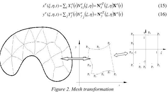
Since the coordinate “z” has been transferred to a dimensionless “” coordinate, and the (0..h) range to (–1..1), futhermore and the h(x,y) gap size independent from z, only the contact area has to be divided into shapes characteristic of a particular 2D element type and then derived into a unified shape by means of conform transfor- mation for numerical integration [4] in order to carry out the integrations.

  

 

 − −

=

=

e

e e

e A e A

d d y

x f dxdy

y x f dxdy y x f

e c c

1 1

1 1

)) , ( ), , ( ( )

, ( )

,

(   J   (14)

40 Szabolcs Szávai–Sándor Kovács

Conform geometry transformation by Legendre shape functions (N) according to [4]

looks like:

( ) ( )

tN

( ) ( )

t X

t

x^e(,, )=_{i i}^e _x^e_i , =N^eT_x , X^e (15)

( )

tN

( ) ( ) ( )

t Y

t

y _j ^eT_y ^e

j ey je

e(,, )= , =N ,Y (16)

Figure 2. Mesh transformation

This integration is carried out in most cases numerically by means of Gaussian quad- rature [4]:

( )

=     

  = =

− − Gi Gj Gi Gj

n i

m

j wGiwGjf d

d

f ,    , ,

1 1 1

1 1

1

J

J (17)

Where _G and _G specified points within the domain of integration and

w

_G are weights at specified points [4].

Legendre shape functions (N) according to [4] have been used for the polynomial approximation of the un-known variables. Only 2D approximation needed for the gap size, deformation and the pressure.

(

t

)

H

( ) ( )

tN

( ) ( )

t

h _{k h}^e_k ^eT_g ^e_g

k e g e

g ,, = , =N ,H ⁽¹⁸⁾

( )

, ,^t =k^H

( ) ( )

^tNk , = ^eTg

( ) ( )

, ^{e t s}=1,2

e k h e e

s _s   _s

 N H (19)

  ^{( ) ( )}

^t

h ^eT_h ^e

rigid e e eg eT g

e H H H N H

N ,1 ^{1 2} = ,













 +

= + (20)

(

t

)

P

( ) ( )

t N

( ) ( )

t

p _l ^eT_p ^e

l e p e l

e,, = , =N ,P (21)

P1 P2

P3

P4

P5 P6

P8

P9

P10

P7

P1 P2

P3

P4

P5 P6 P7

P8

P9

P10

x y





-1

-1 1

1

The variation of the temperature through the thickness has been taken into consider- ation:

(

t

)

_mT_m^e

( )

tN^e_m

( )

^eT

( ) ( )

^e t

e    N  T

 , , , = _ , , = _ , , (22)

Let us note that only the shape functions for the surface nodes, edges and sides of the elements of N on surfaces Sⁱ assume values. Thus the shape functions may be divided into three groups: those related to surfaces S1 and S2 plus the shape function operating inside the lubricant.



₁^{, ,} S₂



T V T S T

T   

 N N N

N = (23)

Accordingly, T may also be grouped similarly:



T V^T _S^T



S T

2 1,T ,T T

T_ = (24)

No shape function is required for the displacement like a rigid body _rigid(t), as it is a parameter associated with the body. For the discretisation of the week integral form of the Reynods equations, the wR weight functions are Np in case of direct solution.

If invers solution is chosen the wR weight function should be Ng. However it has to be considered that the pressure and deformation field are dependent from each other.

The two fields are connected by the solid mechanical description of the surfaces.

Furthermore the pressure distribution has to satisfy the load case as well. For the discretization of the energy equation wQ weight functions are N.

5. VERIFICATION OF DEVELOPED METHOD

The solution of the problem by the p-version finite element method is presented by means of the examples found in the article published by Wolff at all [5] in 1992 as the basis for which the applicability of the solution method constructed here to the problem has been verified. The gap was divided along its length into 15 elements also here. The degree of approximations is given in Table 1.

Table 1 Mesh parameter

Element number 1 2 3 4 5 6 7 8 9 10 11 12 13 14 15

Degree of pressure

approximation 6 6 6 6 6 6 6 6 7 7 7 6 6 6 6

Degree of temperature approximation

4 x 4

4 x 4

4 x 4

4 x 4

4 x 4

4 x 4

4 x 4

4 x 4

4 x 4

4 x 4

4 x 4

4 x 4

4 x 4

4 x 4

4 x 4

42 Szabolcs Szávai–Sándor Kovács

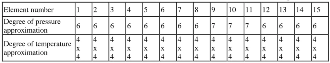
Figure 3. Pressure distribution

for pure rolling Figure 4. Temperature distribution for pure rolling

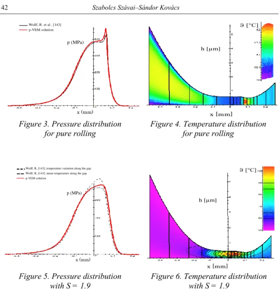
Figure 5. Pressure distribution

with S = 1.9 Figure 6. Temperature distribution with S = 1.9

The calculations were carried out for the state of pure rolling contact and with 1.9 sliding ratio. The elasto-hydrodynamic problem was solved with the use of the opti- mized Newton-Rapshon method [3] and the thermodynamical problem by the atten- uated direct algorithm in iterative manner. The pressure distribution obtained is shown in Figure 3 and Figure 5. The gap size formed as well as the temperature distribution in Figure 4 and Figure 6.

6. IMPLEMENTATION OF EHD PROBLEM TO FEM SOFTWARE

The Comsol Multiphysics software was used for calculating EHD problems. The Comsol Multiphysics uses the finite element formulation with Lagrange test func- tions to solve numerical problems. The weak formulation of the hydrodynamic prob- lem can be created in the Mathematics module and model can be freely modified.

The elastic deformation of the surface and the rigid displacement of the surfaces can

p (MPa) Wolff, R. et al , [143]

p-VEM solution

h (µm10²)

x (mm)

h [µm]

x [mm]

 [°C]

p (MPa) Wolff, R, [143]; temperature variation along the gap Wolff, R, [143]; mean temperature along the gap p-VEM solution

h (µm10²)

x (mm)

h [µm]

x [mm]

 [°C]

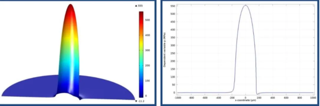
be calculated in the Structural Mechanics module which uses the common structural finite element methods. Since optimized Newton-Rapshon method [3] cannot be adopt to Comsol Multiphysics the solution has been stabilized be Streamline-up- wind/Petrov-Galjorkin and isotropic diffusion method. The results can be seen in Figure 7 and Figure 8.

Figure 7. Pressure distribution of point contact

Figure 8. Surface deformation and subsurface stress distribution

7. CONCLUSION

For the three-dimensional contact problem of lubrication, a two-dimensional lubri- cation fluid film finite element was developed. A remarkable property of this element is that only a two-dimensional mesh has to be maintained. Furthermore, pressure and film thickness can be handled as independent element variables. Integration through the thickness is carried out by making use of dimensionless thickness coordinate.

Three dimensional behaviour of the fluid film temperature can be modelled using higher order approximations through the thickness direction. The method has been verified by line contact and the EHD part has been already implemented to commer- cial FEM software. Implementation of the thermal part is under development.

44 Szabolcs Szávai–Sándor Kovács

ACKNOWLEDGEMENTS

The research was supported by the European Union and the State of Hungary, co- financed by the European Social Fund in the framework of TÁMOP-4.2.4.A/2-11/1- 2012-0001 ‘National Excellence Program’ and National Research, Development and Innovation Office - NKFIH, K115701.

REFERENCES

[1] Carslaw, H. S. & Jaeger, J. C. (1959). Conduction of Heat in Solids. Oxford University Press.

[2] Johnson, K. L. (1987). Contact Mechanics. 2^nd Ed., Cambridge Univ. Press.

[3] Szávai, Sz. & Kovács, S. (2014). P-version FEM model of TEHD lubrication and its implementation to study surface modified contact bodies behaviour.

BALKANTRIB’14: Proceedings, Sinaia, Romania, pp. 716–727.

[4] Páczelt, I. (1999). Finite Element Method in Engineering Practice I. Part (Végeselem-módszer a Mérnöki Gyakorlatban I. Kötet). Miskolc: Miskolci Egyetemi kiadó.

[5] Wolff, R., Nonaka, T., Kubo, A. & Matsuo, K. (1992). Thermal Elastohydro- dynamic Lubrication of Rolling/Sliding Line Contacts. ASME J. of Tribology, Vol. 114, No. 4, pp. 706–713.

Secreteriat of the Vice-Rector for Research and International Relations, University of Miskolc,

Responsible for the Publication: Prof. dr. Tamás Kékesi

Published by the Miskolc University Press under leadership of Attila Szendi Responsible for duplication: Erzsébet Pásztor

Editor: Dr. Ágnes Takács Number of copies printed:

Put the Press in 2018

Number of permission: TNRT–2018– –ME HU ISSN 1785-6892 in print

HU ISSN 2064-7522 online