Efficient computation of matrix power-vector products: application for space-fractional diffusion problems

Efficient computation of matrix power-vector products: application for space-fractional diffusion problems

Ferenc Izsák^a,∗, Béla J. Szekeres^b

aDepartment of Applied Analysis and Computational Mathematics,&MTA ELTE NumNet Research Group, Eötvös Loránd University, Pázmány P. stny. 1C, 1117 - Budapest, Hungary

bDepartment of Numerical Analysis, Eötvös Loránd University, Faculty of Informatics, Pázmány P. stny. 1C, 1117 - Budapest, Hungary

Abstract

A novel algorithm is proposed for computing matrix-vector productsA^αv, whereAis a symmetric positive semidefinite sparse matrix andα > 0. The method can be applied for the efficient implementation of the matrix transformation method to solve space-fractional diffusion problems. The performance of the new algorithm is studied in a comparison with the conventional MATLAB subroutines to compute matrix powers.

Keywords: matrix powers, matrix transformation method, binomial series, space-fractional diffusion 2010 MSC: 65N12, 65N15, 65N30

1. Introduction

In the last two decades, the numerical simulation of (space-) fractional diffusion became an important topic in the numerical PDE’s starting with the poineering paper [1]. Fractional dynamics was observed in a wide range of life sciences [2], earth sciences [3] and financial processes [4]. A frequently used and meaningful mathematical model [5]

of these phenomena is offered by the fractional Laplacian operator [6]. For solving these problems numerically, the so- called matrix transformation method was proposed in [7] and [8]. Accordingly, a mathematical analysis was presented to prove the convergence of this simple approach in case of finite difference [9] and finite element discretization.

The bottleneck of the matrix transformation approach is the computation of the fractional power of the matrices arising from the finite element or the finite difference discretization of the negative Laplacian operators. This is why many authors use a more technical approach [6].

Several algorithms were proposed to compute this matrix power. We refer to the latest approach in [10] and its reference list on the earlier developments. Due to its importance, MATLAB has also a built-in subroutinempower.m.

To bypass this costly procedure, the aim of the present article is to develop a simple and fast numerical method to compute matrix-vector products of type A^αv. This idea was also used in [11] by developing the frequently used Matlab subroutineexpmv.mto compute matrix exponential-vector products.

1.1. Mathematical preliminaries

The main motivation of our study is the efficient numerical solution of the initial-boundary value problem (∂tu(t,x) =−(−∆)^αu(t,x) t∈(0, T), x∈Ω

u(0,x) =u0(x) t∈(0, T), x∈Ω, (1)

where∆ = ∆D or∆ = ∆N denotes the Dirichlet or the Neumann Laplacian on the bounded Lipschitz domainΩand u0∈L2(Ω)is given. Note that−∆⁻¹_D :L2(Ω)→L2(Ω) and−∆⁻¹_N :L2(Ω)/R→L2(Ω)are compact and self-adjoint, so that its fractional power makes sense.

∗Corresponding author

Email addresses: izsakf@cs.elte.hu(Ferenc Izsák),szbpagt@cs.elte.hu(Béla J. Szekeres)

According to thematrix transformation method, (1) can be semidiscretized as

∂tu(t) =−(A)^αu(t) t∈(0, T) (2) whereA is the discretization of the operator−∆D or−∆N either with finite differences or with finite elements.

Accordingly,A∈R^n×n is a symmetric positive semidefinite sparse matrix,v ∈Rⁿ is an arbitrary vector andwe consider the case ofα∈(0,1). The computational challenge is then to compute the productsA^αv, when the solution of (2) is approximated with some explicit time stepping.

If the spectral decomposition ofA is known, such that x₁,x₂, . . . ,x_n are the eigenvectors and λ₁ ≤λ₂ ≤ · · · ≤ λ_n the corresponding eigenvalues of A then A^α has the same eigenvectors, while the corresponding eigenvalues are λ^α₁, λ^α₂, . . . , λ^α_n. Accordingly, ifv=a₁x₁+a₂v₂+· · ·+a_nx_n then

A^αv=a₁λ^α₁x₁+a₂λ^α₂v₂+· · ·+a_nλ^α_nx_n. (3) 2. Main results

2.1. Motivation and main idea

For the first glance, the easiest way to approximate the matrix powerA^αis to truncate thepowerseries A^α= (I+A−I)^α=

∞

X

j=0

α j

(A−I)^j,

whichis satisfied forα >0ifσ(A−I)≤1, where σdenotes the spectral radius. To ensure this, we rather compute A^α=

σ(A) 2

α 2A σ(A)

α

= σ(A)

2

α ∞

X

j=0

α j

2A σ(A)−I

j

. (4)

Using the relation A≥0, for an arbitrary eigenvalueλ˜ of _σ(A)^2A −I we have that−1 =≤λ˜ ≤ ^σ(2A)_σ(A) −1 = 1, so that the binomial series in (4) converges for non-singular matrices A. The convergence, however, is very slow due to the smallest and largest eigenvalues ofA, which are transformed near to−1and1, respectively.

The basic idea is then to apply a spectral decomposition toA: in the subspace ofRⁿ corresponding to the smallest and largest eigenvalues ofA, we apply the direct spectral definition in (3), while in the orthocomplement, the expansion (4) will convergesatisfactorily.

2.2. Method

The decomposition can be formulated by introducing an orthogonal projectionQ:Rⁿ →R^k, which maps to the subspace span

x₁,x₂, . . . ,x_j,x_{n−(k−j−1)}, . . . ,x_n−1,x_n withλ₁≤λ₂≤ · · · ≤λ_j ≤λ_{n−(k−j−1)}≤ · · · ≤λ_n, wherej andkare some parameters. Also, henceforth we focus to the computation ofA^αv,which can be given as

A^αv= σ(A)

2

^α 2A σ(A)

^α v=

σ(A) 2

^α 2A σ(A)

^α Qv+

2A σ(A)

^α

(v−Qv)

. (5)

2.2.1. Computation of the first term in (5)

The projection matrixQin (5) is defined withQ=XX^T and the projectionQv can be given as

Qv=XX^Tv=a1x1+· · ·+ajxj+a_{n−(k−j−1)}x_{n−(k−j−1)}+· · ·+anxn (6) with some coefficientsa₁, a₂, . . . , a_n,where the matrix

X= [x₁,x₂, . . . ,x_j,x_{n−(k−j−1)}, . . . ,x_n−1,x_n]∈R^n×k (7) is composed from the eigenvectors corresponding to the largest and smallest eigenvalues ofA. Observe that, according to the spectral definition of the matrix power in (3), we have

A^αQv=λ^α₁a1x1+· · ·+λ^α_jajxj+λ^α_{n−(k−j−1)}a_{n−(k−j−1)}x_{n−(k−j−1)}+· · ·+λ^α_nanxn=XΛX^Tv, (8) whereΛ is a diagonal matrix with the entriesλ1, . . . , λj, λ_{n−(k−j−1)}, . . . , λn. This gives the first term in (5).

2.2.2. Computation of the second term in (5) We should simply apply here (4) to get

2A σ(A)

^α

(v−Qv) =

∞

X

n=0

α n

2A σ(A)−I

ⁿ

(v−Qv)≈

K

X

n=0

α n

2A σ(A)−I

ⁿ

(v−Qv), (9) where the vectorQvwas already computed in (6). To accelerate the computation in (9) further, we observe that

α n+ 1

2A σ(A)−I

n+1

(v−Qv) = α−j n+ 1

2A σ(A)−I

· α

n

2A σ(A)−I

n

(v−Qv)

,

i.e., a new term in (9) can be computed using only one sparse matrix-vector multiplication.

2.3. Analysis: Estimation for the number of terms in the Taylor expansion (9) The accuracy of the approximation in (9) will be given using the error indicator

µ_max=

2A σ(A)−I

(I−Q)

= max

2λ_j+1 σ(A) −1

;

2λ_n−k+j σ(A) −1

= max

1−2λ_j+1

σ(A);2λ_n−k+j σ(A) −1

,

which measures the error of the truncation in (9) and can be decreased by choosing suitable (large enough) parameters j andk.

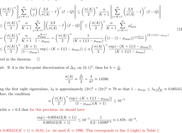
Theorem 1. Assume that the eigenvaluesforX in (7)and the eigenvectorsforΛ in (8)are computed exactly. Then an upper bound for computational error inA^αv is the term

α σ(A)

2

^αexp (−(K+ 1)(1−µmax)) (K+ 1)(1−µmax) kvk.

In practice, to ensure a precision εof A^αv , the numberK of the terms in (9)should satisfy

K≤ 1

1−µmax

G ε

α 2

σ(A) ^α

−1,

whereG is the inverse of the function R⁺3s7→ ^e−s_s .

Proof:The computational error inA^αvcan be expressed in the following form.

A^αv−



A^αQv+ σ(A)

2

α K

X

j=0

α j

2A σ(A)−I

j

(v−Qv)





=



A^α− σ(A)

2

α K

X

j=0

α j

2A σ(A)−I

j

(v−Qv) = σ(A)

2

α ∞

X

j=K+1

α j

2A σ(A)−I

j

(I−Q)v.

(10)

Therefore, we first derive an upper bound for the matrix series in the last line. Observe that 2A

σ(A)−I ^j

(I−Q)v= 2A

σ(A)−I ^j

(I−Q)^jv=

2A σ(A)−I

(I−Q) ^j

v. (11)

Since we use symmetric matrices, the matrix norm k · k in the following refers both to the spectral norm and the l₂-norm. Since0< α <1, we easily get the inequality

α j

=

α j−1

α−j+ 1 j

≤

α j−1

j−1

j ≤

α j−2

j−1 j

j−2

j−1 ≤ · · · ≤

α 0

α j =α

j,

which can be used in (10) with (11) to get the following estimate σ(A)

2 ^α

∞

X

j=K+1

α j

2A σ(A)−I

^j

(I−Q)

≤ σ(A)

2

^α α K+ 1

∞

X

j=K+1

2A σ(A)−I

^j

(I−Q)

≤ σ(A)

2

^α α K+ 1

∞

X

j=K+1

2A σ(A)−I

(I−Q)

j

≤ σ(A)

2

^α α K+ 1

∞

X

j=K+1

µ^j_max

= σ(A)

2

^α α

K+ 1· µ^K+1_max 1−µ_max =

σ(A) 2

^α 1

(K+ 1)(1−µ_max)

(1−(1−µ_max))^1−µ1max(K+1)(1−µmax)

≤ σ(A)

2

^α (K+ 1)

(1−µmax)exp (−(K+ 1)(1−µmax))≤α σ(A)

2

^αexp (−(K+ 1)(1−µmax)) (K+ 1)(1−µmax) ,

(12)

as stated in the theorem.

Example. IfAis the five-point discretization of∆N on(0,1)², then forh= ₆₀¹ σ(A)

2 ≈

8 h²

2 = 4

h² ≈14590.

Ignoring the first eight eigenvalues, λ₉ is approximately (2π)²+ (2π)² ≈79so that 1−µ_max ≤λ_9σ(A)² ≈0.005412.

Therefore, the condition

α σ(A)

2 α

exp (−(K+ 1)(1−µmax))

(1−µmax)(K+ 1) ≤10⁻⁵ gives withα= 0.3that for this precision, we should have

exp (−0.005412(K+ 1))

0.005412(K+ 1) ≤10⁻⁵ 1

0.3·14590^0.3 ≈1.878·10⁻⁶,

so that0.005412(K+ 1)≈10.81, i.e. we needK≈1996. This corresponds to line 3 (right) in Table 1.

2.4. Numerical experiments

In the experiments, the matrix A is the five-point finite difference approximation of −∆_N on (0,1)^d using N uniformly distributed grid points in one direction. We measure the CPU time and the memory usage of the different approaches. To investigate the accuracy, we use the error indicatorr=kA^1−αA^αv−Avkmax with a random vector v. The CPU time and the error indicator are computed from the average of ten independent runs.

2.4.1. Experimental analysis of our method

The main parameters in the algorithm of Section 2.2 are the following. N: the number of the grid points in one direction; k: the number of the eigenvectors used to the computation in the first term (6); j: the number of the smallest eigenvectors among thekextreme ones;K: the number of the terms in the Taylor approximation in (9);res:

the residual inchdav.mfor approximating the eigenvectors and eigenvalues (the default value is10⁻⁸).

Table 1: Performance of the method in Section 2.2 using the error indicatorrwithN= 60, d= 2andα= 0.3.

k j K time [s] r res k j K time [s] r res

20 10 20 0.544 13.3 10⁻⁸ 40 20 2000 1.21 1.88·10⁻⁴ 10⁻⁸ 20 10 200 0.526 9.75·10⁻³ 10⁻⁸ 40 20 20000 1.78 2.36·10⁻⁴ 10⁻⁸ 20 10 2000 0.568 1.88·10⁻⁴ 10⁻⁸ 16 8 2000 0.44 1.72·10⁻⁵ 10⁻¹⁴ 20 10 20000 1.23 2.00·10⁻⁴ 10⁻⁸ 12 6 2000 0.36 2.05·10⁻⁵ 10⁻¹⁴ 20 10 200000 8.88 1.96·10⁻⁴ 10⁻⁸ 16 8 20000 1.16 1.91·10⁻¹⁰ 10⁻¹⁴

The experiments confirm some of our expectations:

It is necessary to compute both the smallest and the largest eigenvalues. If the set{2λ_j/σ(A)−1 :j= 1,2, . . . , n}is symmetric, then the optimal choice isj= ^k₂.

The convergence of the Taylor series in (9) is slow: we need at least a few hundred terms to get an acceptable accuracy. See lines 1-4(left)in Table 1. The result in line 3(left)confirms our estimation in the example.

The optimal number ofk is a few tens. For larger values ofk, the computation becomes slow and the inaccurate eigenstructure results in a relatively large error contributions to (8). The decomposition in (5) becomes then also inaccurate, such that increasingk further gives an even worse approximation. Seethelines fork= 40in Table 1.

A cornerstone of the algorithm in Section 2.2 is an efficient eigensolver. We compared the performance of the built-in Matlab subroutine eigs.mand the special subroutinesjdcg.m(see [12]),chdav.m (see [13] and its improved version bchdav.m. For matrices of moderate sizes (up to a few thousands of non-zero elements), all subroutines perform equally well. For large 2-dimensional cases,eigs.mbecame the most efficient with an appropriate setting of the tolerance and the iteration number in the algorithm. For large 3-dimensional cases, if multiple eigenvalues are expected, we advice to use the bchdav.msubroutine. An experimental comparison of the effect of these eigensolvers can be found in Table 2.

Table 2: Performance of the method in Section 2.2 using different eigensolvers using the error indicatorrwithα= 0.3.

N eigs.m jdcg.m chdav.m bchdav.m

r time [s] r time [s] r time [s] r time [s]

2-dimensional case

20 2.9·10⁻¹² 0.26 1.9·10⁻¹² 0.27 2·10⁻¹² 0.25 1.8·10⁻¹² 0.28 40 8.6·10⁻¹² 0.44 1.1·10⁻¹¹ 1.4 1.2·10⁻¹² 0.94 1.1·10⁻¹¹ 0.76 100 6.7·10⁻¹² 4.9 5.3·10⁻³ 4.3 1.7·10⁻¹⁰ 10 1.3·10⁻¹⁰ 11.2

3-dimensional case

20 3.1·10⁻¹² 2.3 3.7·10⁻¹² 3.9 3.7·10⁻¹² 2.4 3.7·10⁻¹² 2 30 1·10⁻¹¹ 13.8 9.9·10⁻¹¹ 18.9 7.6·10⁻¹² 11.8 8.9·10⁻¹² 15 40 1.8·10⁻¹¹ 86 1.9·10⁻¹¹ 69 1.8·10⁻¹¹ 43 1.9·10⁻¹¹ 38

2.4.2. Comparison with the standard method in 3-dimensional case

Since the real computational challenge is to deal with 3-dimensional problems, we focus now on this case. Our approach to computeA^αvdirectly is compared now with the standard way: computingA^αfirst (over time t1) using thempower.msubroutine and multiplyingA^αwithv(over time t2) forα= 0.3. Results are displayed in Table 3.

Table 3: Performance of the method in Section 2.2 with different parameters using the error indicatorrwithd= 3andα= 0.3.

conventional method proposed method

N t1[s] t2[s] memory[MB] precision j time[s] memory[MB] precision 10 0.28 0.002 16 2.1·10⁻¹¹ 8 0.132 0.12 5.2·10⁻¹² 20 145.9 0.80 1·10³ 5.9·10⁻¹⁰ 8 0.84 0.99 2.6·10⁻¹¹ 25 1251 128 2.6·10³ 4.5·10⁻¹¹ 8 3.32 5 7.9·10⁻¹² 30 7.6·10⁵ 370 1.5·10⁴ 1.1·10⁻¹¹ 8 6.75 8 8.2·10⁻¹¹

35 - - overflow - 8 8.84 16 5.85·10⁻¹¹

40 - - overflow - 8 20.68 30 6.83·10⁻⁷

3. Conclusions

The present algorithm to compute matrix power-vector products completes the favor of using matrix transformation methods, which delivers an elegant and easily accessible scheme and optimal convergence rate for the finite element and finite difference discretization of space-fractional diffusion problems. Also, as pointed out in the present work, a fast numerical procedure can be constructed to solve the fully discrete schemes using explicit time stepping.

Acknowledgments

The first author was supported by the Hungarian Research Fund OTKA (grant 112157). The project has been supported by the European Union, co-financed by the European Social Fund. EFOP-3.6.1-16-2016-0023.

References

[1] M. M. Meerschaert, C. Tadjeran, Finite difference approximations for fractional advection-dispersion flow equa- tions, J. Comput. Appl. Math. 172 (1) (2004) 65–77. doi:10.1016/j.cam.2004.01.033.

[2] C. Bucur, E. Valdinoci, Nonlocal diffusion and applications, Vol. 20 of Lecture Notes of the Unione Matematica Italiana, Springer, [Cham]; Unione Matematica Italiana, Bologna, 2016. doi:10.1007/978-3-319-28739-3.

[3] Y. Zhang, H. Sun, H. H. Stowell, M. Zayernouri, S. E. Hansen, A review of applications of fractional calculus in Earth system dynamics, Chaos Solitons Fractals 102 (2017) 29–46. doi:10.1016/j.chaos.2017.03.051.

[4] S. Z. Levendorski˘ı, Pricing of the American put under Lévy processes, Int. J. Theor. Appl. Finance 7 (3) (2004) 303–335. doi:10.1142/S0219024904002463.

[5] F. Izsák, B. J. Szekeres, Models of space-fractional diffusion: a critical review, Appl. Math. Lett. 71 (2017) 38–43.

doi:10.1016/j.aml.2017.03.006.

[6] R. H. Nochetto, E. Otárola, A. J. Salgado, A PDE approach to fractional diffusion in general domains: a priori error analysis, Found. Comput. Math. 15 (2015) 733–791. doi:10.1007/s10208-014-9208-x.

[7] M. Ilić, F. Liu, I. Turner, V. Anh, Numerical approximation of a fractional-in-space diffusion equation. I, Fract.

Calc. Appl. Anal. 8 (3) (2005) 323–341.

[8] M. Ilić, F. Liu, I. Turner, V. Anh, Numerical approximation of a fractional-in-space diffusion equation. II. With nonhomogeneous boundary conditions, Fract. Calc. Appl. Anal. 9 (4) (2006) 333–349.

[9] B. J. Szekeres, F. Izsák, Finite difference approximation of space-fractional diffusion problems: The matrix transformation method, Comput. Math. Appl. 73 (2) (2017) 261–269. doi:10.1016/j.camwa.2016.11.021.

[10] N. J. Higham, L. Lin, An improved Schur-Padé algorithm for fractional powers of a matrix and their Fréchet derivatives, SIAM J. Matrix Anal. Appl. 34 (3) (2013) 1341–1360. doi:10.1137/130906118.

[11] A. H. Al-Mohy, N. J. Higham, Computing the action of the matrix exponential, with an application to exponential integrators, SIAM J. Sci. Comput. 33 (2) (2011) 488–511. doi:10.1137/100788860.

[12] Y. Notay, Combination of Jacobi-Davidson and conjugate gradients for the partial symmetric eigenproblem, Numer. Linear Algebra Appl. 9 (1) (2002) 21–44.

[13] Y. Zhou, Y. Saad, A Chebyshev–Davidson algorithm for large symmetric eigenproblems, SIAM J. Matrix Anal.

Appl. 29 (3) (2007) 954–971. doi:10.1137/050630404.