Evaluation of Deep Learning Strategies for Nucleus Segmentation in Fluorescence Images
Juan C. Caicedo,
1Jonathan Roth,
1,2Allen Goodman,
1Tim Becker,
1Kyle W. Karhohs,
1Matthieu Broisin,
1,3Csaba Molnar,
1,4Claire McQuin,
1Shantanu Singh,
1Fabian J. Theis,
2Anne E. Carpenter
1*
Abstract
Identifying nuclei is often a criticalfirst step in analyzing microscopy images of cells and classical image processing algorithms are most commonly used for this task.
Recent developments in deep learning can yield superior accuracy, but typical evalua- tion metrics for nucleus segmentation do not satisfactorily capture error modes that are relevant in cellular images. We present an evaluation framework to measure accu- racy, types of errors, and computational efficiency; and use it to compare deep learning strategies and classical approaches. We publicly release a set of 23,165 manually anno- tated nuclei and source code to reproduce experiments and run the proposed evalua- tion methodology. Our evaluation framework shows that deep learning improves accuracy and can reduce the number of biologically relevant errors by half. © 2019 The Authors.Cytometry Part Apublished by Wiley Periodicals, Inc. on behalf of International Society for Advancement of Cytometry.
Key terms
fluorescence imaging; image analysis; deep learning; nuclear segmentation; chemical screen.
Image analysis is a powerful tool in cell biology to collect quantitative measurements in time and space with precision, speed, and sensitivity. From image-based assays to high-content screening (1,2), microscopy images have led to understanding genetic perturbations, pursuing drug discovery, and phenotyping cells in biomedical applica- tions and cell biology research (3,4). The most widely used quantitative imaging technique in biological laboratories isfluorescence imaging; with automation it can easily produce terabytes of primary research data (5). Accurate and automated anal- ysis methods are key to successfully quantify relevant biology in such large image collections.
One critical step in quantifyingfluorescence images is often the identification of the nucleus of each cell with a DNA stain, and there is a long history of research efforts to design and improve nuclear and cellular segmentation (6). One of the most commonly used strategies for nucleus segmentation is Otsu’s thresholding method (7) followed by seeded watershed (8,9), because of its effectiveness, simplicity of use and computational efficiency. Machine learning-based segmentation methods have also been introduced for segmenting cells (10), which typically require annotated examples in the form of segmentation masks or interactive scribbles. Many of these strategies are readily available in various bioimage software packages (11), including open source options such as CellProfiler (12), Ilastik (10), and ImageJ/Fiji (13), facil- itating their adoption in routine biological research.
Despite widespread adoption, segmentation tools in biology generally do yield nontrivial amounts of segmentation error. These may silently propagate to
1Imaging Platform, Broad Institute of MIT and Harvard, Cambridge, Massachusetts
2Institute of Computational Biology, German Research Center for
Environmental Health, Munich, Germany
3Biomedical Imaging Group, Ecole polytechnique fédérale de Lausanne, Lausanne, Switzerland
4Biological Research Centre of the Hungarian Academy of Sciences, Szeged, Hungary
Received 9 July 2018; Revised 31 May 2019; Accepted 23 June 2019 Grant sponsor: European Union; Grant sponsor: National Institutes of Health;
Grant sponsor: National Institute of Gen- eral Medical Sciences
Additional Supporting Information may be found in the online version of this article.
*Correspondence to: Anne E. Carpenter, Imaging Platform, Broad Institute of MIT and Harvard, 415 Main Street,
Cambridge, MA 02142.
Email: anne@broadinstitute.org Published online 16 July 2019 in Wiley Online Library (wileyonlinelibrary.com) DOI: 10.1002/cyto.a.23863
© 2019 The Authors.Cytometry Part A published by Wiley Periodicals, Inc. on behalf of International Society for Advancement of Cytometry.
This is an open access article under the terms of the Creative Commons Attribution-NonCommercial License, which permits use, distribution and reproduction in any medium, provided the original work is properly cited and is not used for commercial purposes.
Cytometry Part A95A: 952–965, 2019
downstream analyses, yielding unreliable measures or sys- temic noise that is difficult to quantify and factor out. There are several causes for segmentation errors. First, existing algo- rithms have limitations due to the assumptions made in the computational design that do not always hold, such as thresholding methods that assume bimodal intensity distribu- tions, or region growing that expects clearly separable bound- aries. Second, the most popular solutions for nucleus segmentation were originally formulated and adopted several decades ago when the biological systems and phenotypes of interest were often simpler; however, as biology pushes the limits of high-throughput cellular and tissue models, natural and subtle variations of biologically meaningful phenotypes are more challenging to segment. Finally, algorithms are usu- ally configured using a few—hopefully representative—images from the experiment, but variations in signal quality and the presence of noise pose challenges to the robustness and reli- ability of the solution at large scale.
The ideal approach to nucleus segmentation would be a generic, robust, and fully automated solution that is as reliable as modern face detection technologies deployed in mobile applications and social networks. The current state of the art in face detection and many other computer vision tasks is based on deep learning (14), which has demonstrated high accuracy, even surpassing human-level performance in certain tasks (15). Several models based on deep learning have already been proposed for cell segmentation in biological applications, most notably U-Net (16) and DeepCell (17), which are based on convolutional neural networks (CNNs).
In this article, we present an evaluation framework, including a new metric, to answer the question of how much improvement is obtained when adopting deep learning models for nucleus segmentation. The most commonly-used metric for nucleus/cell segmentation evaluation is the Jaccard index (17–19), which measures pixel-wise overlap between ground truth and segmentations estimated by an algorithm. From a cell biology perspective, pixel-wise overlap alone is not useful to diagnose the errors that actually impact the downstream analysis, such as missing and merged objects (Fig. S1). Thus, we recommend the use of metrics that explicitly count cor- rectly segmented objects as true positives and penalize any instance-level error, similar to practice in diagnostic applica- tions (20,21). These include object-level F1-score and false pos- itives, among others.
We demonstrate the utility of this methodology by evalu- ating two deep learning methods proposed for cell segmenta- tion and comparing them against classical machine learning and image processing algorithms. The goal of our study is to investigate the potential of deep learning algorithms to improve the accuracy of nucleus segmentation influorescence images. Expert biologists on our team hand-annotated more than 20,000 nuclei in an image collection of 200 images of the DNA channel from a large image-based chemical screen, sampled from a diverse set of treatments (22). We apply our evaluation framework to analyze different types of segmenta- tion errors, computational efficiency, and the impact of
quantity and quality of training data for creating deep learn- ing models.
Our study is restricted to segmenting the nucleus of cells influorescence images, which is different from the more gen- eral cell segmentation problem. We also assume the availability of a large dataset of annotated images for training the machine learning models. We note that the deep learning techniques evaluated in our experiments were designed for different set- tings: general purpose cell segmentation with limited training data. Nevertheless, both deep learning methods (DeepCell and U-Net) showed improved ability for segmenting nuclei andfix errors that are relevant to experimental biology when trained with a large image set.
M
ATERIALSImage Collection
The image set is a high-throughput experiment of chemical perturbations on U2OS cells, comprising 1,600 bioactive com- pounds (22). The effect of treatments was imaged using the Cell Painting assay (23) which labels cell structures using six stains, including Hoechst for nuclei. From this image collec- tion, we randomly sampled 200 fields of view of the DNA channel, each selected from a different compound. By doing so, phenotypes induced by 200 distinct chemical perturba- tions were sampled.
The original image collection is part of the Broad Bioimage Benchmark Collection, with accession number BBBC022, and the subset used for this study has been made publicly available with accession number BBBC039 at https://
data.broadinstitute.org/bbbc/BBBC039/.
Expert Annotations
Each image in the sampled subset was reviewed and manually annotated by PhD-level expert biologists. Annotators were made to label each single nucleus as a distinguishable object, even if nuclei happen to be clumped together or appear to be touching each other. Nuclei of all sizes and shapes were included as our goal was to densely annotate every single nucleus that can be recognized in the sampled images, regard- less of its phenotype. In this way, a wide variety of pheno- types was covered, including micronuclei, toroid nuclei, fragmented nuclei, round nuclei, and elongated nuclei, among others (22).
We included tiny fragments of nuclei as part of the annotated objects in our dataset, which correspond to small blobs of DNA-stained material that appear to be membrane bound, primarily micronuclei. The biological relevance of micronuclei is abundantly documented in the literature (24–29) and these are frequently quantified usingfluorescent imaging for projects involving cancer research, congenital dis- orders, and therapy toxicity, among others. Adding these tiny objects to the dataset is useful to stimulate computational research that detects and quantifies them better.
Creating a resource of manually annotated images is time consuming, and existing tools for annotating natural images are not ideal for microscopy. In order to improve and
simplify the image annotation experience for experts in our team, we created a prototype annotation tool to assign single-object masks in images. Our user interface allowed the experts to zoom in and out to double check details, and also presented the annotation masks overlaid on top of the original image using a configurable transparency layer. Importantly, our annotation tool was based on assisted segmentation based on superpixels, which are computed on intensity features to facili- tate user interactions.
Our prototype tool was useful to collect nucleus annota- tions for this research; however, significant development is needed to improve it. Alternative methods for collecting image annotations now exist, such as the Quanti.us system (30) for distributing manual annotations to nonexpert workers on the internet. This may enable the annotation process for new projects to be scaled up quickly to many more images, and, according to their findings, reaching similar precision to experts when multiple workers provide independent annotation replicates.
M
ETHODSIdentifying nuclei in an image is best framed as an“instance segmentation”problem (31), where the challenge is tofind dis- tinct regions corresponding to a single class of objects: the nucleus. Semantic segmentation (32), which splits an image to regions of various classes without requiring objects to be sepa- rated, is not helpful for nucleus segmentation because there is only one class, and touching nuclei would not be distinguished
from each other. Both of the deep learning strategies evaluated in this article are cases of instance segmentation that formulate nucleus segmentation as a boundary detection problem.
The boundary detection problem consists of identifying three different types of pixels in an image of nuclei:
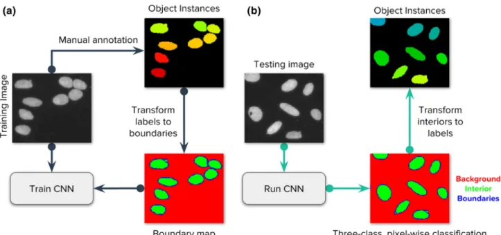
(a) background, (b) interior of nuclei, and (c) boundaries of nuclei. This formulation simplifies the problem of instance segmentation into a three-class, pixel-wise classification prob- lem (Fig. 1), which can be understood as a semantic segmen- tation solution to identify the structural elements of the image. The critical class to separate single objects is the boundary class: failure to classify boundaries correctly will result in merged or split objects. The actual segmentation masks are obtained from the interior class, which covers the regions where objects are located. This requires additional postprocessing steps over classification probability maps to recover individual instances using the connected components algorithm (33) and morphological operators (34) (Supporting Information S2). Note that while we pose this as a pixel-wise classification problem of boundaries, we evaluate the perfor- mance on the success of identifying entire objects.
The ground truth to solve the boundary detection prob- lem starts with masks individually assigned to each object (Section 2.2) and then transformed to three-class annota- tions. The boundary annotations are initially obtained from ground truth annotations using a single pixel contour around each nucleus. We then expand this contour with two more pixels, one inside and another outside the boundary to cover natural pixel intensity variations of the input image
Figure 1.Strategy of the evaluated deep learning approaches. Our main goal is to follow the popular strategy of segmenting each nucleus and micronucleus as a distinct entity, regardless of whether it shares the same cell body with another nucleus. It is generally possible to group nuclei within a single cell using other channels of information in a postprocessing step if the assay requires it. (a) Images of the DNA channel are manually annotated, labeling each nucleus as a separate object. Then, labeled instances are transformed to masks for background, nucleus interior, and boundaries. A convolutional neural network (CNN) is trained using the images and their corresponding masks. (b) The trained CNN generates predictions for the three class classification problem. Each pixel belongs to only one of the three categories. In postprocessing, the predicted boundary mask is used to identify each individual instance of a nucleus. [Colorfigure can be viewed at wileyonlinelibrary.com]
and also to compensate for errors in manual annotations.
We tested with boundaries of different sizes but did not observe any significant benefits of further adjusting this configuration.
Various CNNs can be used for nucleus segmentation, including the Mask-RCNN model (35), which decomposes images into regionsfirst and then predicts object masks. The automatic design of neural networks by searching the space of architectures with an optimization procedure (36) may also be used to create generic nucleus segmentation networks. How- ever, in this work we do not propose novel architectures, instead, we develop an evaluation methodology to identify errors and improve performance of existing models. Specifi- cally, we evaluate two architectures, representing two promi- nent models designed and optimized for segmenting biological images: DeepCell (17) and U-Net (16). We use the same preprocessing and postprocessing pipeline when evaluating both CNN models (Supporting Information S2), so differences in performance are explained by architectural choices only.
DeepCell
DeepCell (17) is a framework designed to perform general- purpose biological image segmentation using neural networks.
Its driving philosophy is to get deep learning operational in biological laboratories using well-constructed models that can be trained with small datasets using modest hardware require- ments, making them usable in a small data regime. The DeepCell library is open source and features a Docker con- tainer with guidelines for training and testing models with new data via Jupyter Notebooks, and more recently, user- friendly functionalities to run a deep learning application in the cloud (37).
The DeepCell model evaluated in our work is a CNN that segments images of cells using a patch-based, single pixel classification objective. The network architecture has seven convolutional layers, each equipped with a ReLu nonlinearity (38) and batch normalization (39); three max-pooling layers to progressively reduce the spatial support of feature maps;
and two fully connected layers; totaling about 2.5 million trainable parameters per network (a full DeepCell model is an ensemble offive networks). Note that DeepCell was designed to be trained in a sample wise fashion and then executed in a fully convolutional way. During training, the incoming feature layer isflattened, and during execution a tensor product using the same weight matrix is used. This architecture has a recep- tive field of 61×61 pixels, which is the approximate area needed to cover a single cell (of a diameter up to 40μm, imaged at 20× at a resolution of 0.656μm/pixel), and pro- duces as output a three-class probability distribution for the pixel centered in the patch.
In our evaluation, we use the recommended configura- tion reported by Van Valen et al. (17), which was demon- strated to be accurate on a variety of cell segmentation tasks, including mammalian cell segmentation and nuclei. Their configuration include training an ensemble of five replicate networks to make predictions in images. Thefinal segmenta- tion mask is the average of the outputs produced by each
individual network. The ensemble increases processing time and the number of trainable parameters, but can also improve segmentation accuracy. The settings of the DeepCell system that we used in our experiments can be reproduced using the following Docker container: https://hub.docker.com/r/
jccaicedo/deepcell/.
U-Net
The U-Net architecture (16) resembles an autoencoder (40) with two main sub-structures: (a) an encoder, which takes an input image and reduces its spatial resolution through multi- ple convolutional layers to create a representation encoding.
(b) A decoder, which takes the representation encoding and increases spatial resolution back to produce a reconstructed image as output. The U-Net introduces two innovations to this architecture: First, the objective function is set to recon- struct a segmentation mask using a classification loss; and second, the convolutional layers of the encoder are connected to the corresponding layers of the same resolution in the decoder using skip connections.
The U-Net evaluated in our work consists of eight con- volutional layers and three max pooling layers in the encoder branch, and eight equivalent convolutional layers with upscaling layers in the decoder branch. We note that batch normalization layers were not part of the original U-Net design, so we added one after all convolutional layers in our implementation. The skip connections copy the feature maps from the encoder to the decoder. The receptive field of the U-Net is set to 256×256 pixels during training, which can cover a large group of cells at the same time. This architecture has a total of 7.7 million trainable parameters.
We adapted the objective function as a weighted classifi- cation loss, giving 10 times more importance to the boundary class. We did not introduce a different weighting scheme for edges between two cells, giving all boundary pixels the same weight regardless of their context (background or another cell). We apply basic data augmentation during training, including random cropping,flips, 90rotations, and illumina- tion variations. Also, we apply additional data augmentation using elastic deformations, as discussed by the authors (16).
The training parameters for this network were tuned using the training and validation sets, and thefinal model is applied to the test set to report performance. The source code of our U-Net implementation can be found in https://github.com/
carpenterlab/2019_caicedo_cytometryA, with an optional CellProfiler 3.0 plugin of this nucleus-specific model (41).
Also, a U-Net plugin was independently developed for ImageJ for running generic cell segmentation and quantification tasks (42).
Evaluation Metrics
Measuring the performance of cell segmentation has been generally approached as measuring the difference between two segmentation masks: a reference mask with ground truth objects representing the true segmentation, versus the pre- dicted/estimated segmentation mask. These metrics include root-mean-square deviation (43), Jaccard index (17), and
bivariate similarity index (18), among others. However, these metrics focus on evaluating pixel-wise segmentation accuracy only, and fail to quantify object-level errors explicitly (such as missed or merged objects).
In our evaluation, we adopt an object-based accuracy metric that uses a measure of area coverage to identify cor- rectly segmented nuclei. Intuitively, the metric counts the number of single objects that have been correctly separated from the rest using a minimum area coverage threshold. The metric relies on the computation of intersection-over-union between ground truth objectsTand estimated objectsE:
IoU Tð ,EÞ=T\E T[E
Consider n true objects and m estimated objects in an image. A matrix Cn×m is computed with all IoU scores between true objects and estimated objects to identify the best pairing. This is a very sparse matrix because only a few pairs share enough common area to score a nonzeroIoUvalue.
To complete the assignment, a threshold greater than 0.5 IoUis applied to the matrix to identify segmentation matches.
In our evaluation, we do not accept overlapping objects, that is, one pixel belongs only to a single nucleus. Thus, a threshold greater than 0.5 ensures that for each nucleus in the ground truth there is no more than one match in the predictions, and vice versa. We also interpret this threshold as requiring that at least half of the nucleus is covered by the estimated segmenta- tion to call it a true positive. In other words, segmentations smaller than half the target object are unacceptable, raising the bar for practical solutions. This differs from a previous strategy (44) that takes a similar approach but does not impose this constraint, potentially allowing for very low object coverage.
At a given IoU threshold t, the object-based segmentation F1-score is then computed as:
F1= 2TP 2TP+FN+FP:
We compute the averageF1-score across all images, and then across multiple thresholds, starting at t = 0.50 up to t = 0.90 with incrementsΔt = 0.05. This score summarizes the quality of segmentations by simultaneously looking at the proportion of correctly identified objects as well as the pixel- wise accuracy of their estimated masks.
Our evaluation metric is similar in spirit to other evalua- tion metrics used in computer vision problems, such as object detection in the PASCAL challenge (45) and instance seg- mentation in the COCO challenge (31,46). One important difference between these metrics and ours is that our problem considers a single object category (the nucleus), and therefore, it is more convenient to adopt theF1-score instead of preci- sion. Precision and recall have been used in previous studies of nucleus segmentation in fluorescent images (47), and F1-score has also been adopted to measure segmentation per- formance in tissue samples (48). But we note that our score is evaluated across multiple intersection-over-union thresholds,
which is the practice in modern computer vision research to simultaneously measure object detection accuracy as well as shape alignment accuracy.
In our evaluation, we also measure other quality metrics, including the number and type of errors to facilitate perfor- mance analysis (49). The following are different types of errors that a segmentation algorithm can make: false nega- tives (missed objects); merges (under-segmentations), which are identified by several true objects being covered by a single estimated mask; and splits (over-segmentations), which are identified by a single true object being covered by multiple estimated masks. We identify these errors in the matrixCof IoU scores using a fixed threshold for evaluation, and keep track of them to understand the difficulties of an algorithm to successfully segment an image.
Baseline Segmentations Classic image processing
We use CellProfiler 3.0 (41) pipelines to create baseline seg- mentations. CellProfiler was used as a baseline over other tools because it offers greatflexibility to configure multi-step image processing pipelines that connect different algorithms for image analysis, and it is widely used in biology labs and high-throughput microscopy facilities. The pipelines are con- figured and tested by an expert image analyst using images from the training set, and then run in the validation and test set for evaluation. We refer to two CellProfiler pipelines for obtaining baseline segmentations: basic and advanced.
The basic pipeline relies only on the configuration of the module IdentifyPrimaryObjects, which is frequently used to identify nuclei. The module combines thresholding tech- niques with area and shape rules to separate andfilter objects of interest. This is the simplest way of segmenting nuclei images when the user does not have extensive experience with image analysis operations, yet it is complete enough to allow them to configure various critical parameters.
The advanced pipeline incorporates other modules for preprocessing the inputs and postprocessing the outputs of theIdentifyPrimaryObjectsmodule. In our advanced configu- ration, we included illumination correction, median filters and opening operations, to enhance and suppress features in the input images before applying thresholding. These opera- tions are useful to remove noise and prepare images to the same standard for segmentation using the same configuration.
The postprocessing steps include measuring objects to apply additionalfilters and generate the output masks.
A single pipeline was used for segmenting images in the BBBC039 dataset, while Van Valen’s set required to split the workflow in two different pipelines. We observed large signal variation in Van Valen’s set given that these images come from different experiments and reflect realistic acquisition modes. Two settings were needed for thresholding, the first for normal single mode pixel intensity distributions and another one for bimodal distributions. The latter is applied to cases where subpopulations of nuclei are significantly brighter than the rest, requiring two thresholds. We used a clustering approach to automatically decide which images needed which
pipeline. The pipelines used in our experiments are released together with the data and code.
Segmentation using classic machine learning
We used Ilastik (10) to train a supervised machine-learning model as an additional benchmark in this evaluation. Ilastik is effective at balancing memory and CPU requirements, allowing users to run segmentations in real time with sparse annotations over the images (scribbles). We loaded the full set of existing annotated training images, and trained a Random Forest classi- fier with the default parameters. The feature set included inten- sity, edge, and texture features in three different scales. The annotated images used the same three categories used for deep-learning-based segmentation: background, interior, and boundaries of nuclei. In addition, we subsampled pixels in the background and interior categories to balance annotations and reduce the impact of redundant pixels.
After the Random Forest model is trained, the validation and test images were loaded into Ilastik for predictions. We obtained the probability maps for each category and applied the same postprocessing steps used for deep-learning-based segmentations (Supporting Information S2).
R
ESULTSDeep Learning Improves Nucleus Segmentation Accuracy
Overall, wefind that deep learning models exhibit higher accu- racy than classical segmentation algorithms, both in terms of
the number of correctly identified objects, as well as the locali- zation of boundaries of each nucleus (Fig. 2). We evaluate these properties using theF1-score (the harmonic average of preci- sion and recall) averaged over increasingly stringent thresholds of overlap between the ground truth and prediction. U-Net and DeepCell obtained higher average F1-scores (Fig. S1), yielding 0.898 and 0.858, respectively, versus 0.840 for Random Forests, 0.811 for advanced CellProfiler and 0.790 for the basic CellProfiler pipeline. This improvement is a significant margin when experiments are run at large scale with thousands of images. Deep learning models yield a higher average F1-score across higher thresholds (Fig. 2a), indicating that the bound- aries of objects are more precisely mapped to the correct con- tours compared to the other methods.
The most common errors for all methods are merged objects, which occur when the segmentation fails to separate two or more touching nuclei (yellow arrows in Fig. 2b). Deep learning strategies tend to reduce this type of error (more in Fig. 3c) and provide tighter and smoother segmentation boundaries than those estimated by global Otsu thresholding and declumping, which is at the core of the baseline Cel- lProfiler pipelines for nucleus segmentation.
Qualitatively, nucleus boundaries predicted by deep learning appear to define objects better than those produced by human annotators using an assistive annotation tool, which can introduce boundary artifacts. Neural nets can learn to provide edges closer to the nuclei with fewer gaps and better-delineated shapes, despite being trained with examples
Figure 2. Segmentation performance offive strategies compared against ground-truth expert segmentations. (a) AverageF1-score versus nucleus coverage for U-Net (green), DeepCell (yellow), Random Forest (purple), CellProfiler advanced (red), and CellProfiler basic (blue).
Theyaxis is averageF1-score (higher is better), which measures the proportion of correctly segmented objects. Thexaxis represents intersection-over-union (IoU) thresholds as a measurement of how well aligned the ground truth and estimated segmentations must be to count a correctly detected nucleus. Higher thresholds indicate stricter boundary matching. Notice that averageF1-scores remain nearly constant up to IoU = 0.80; at higher thresholds, performance decreases sharply, which indicates that the proportion of correctly segmented objects decreases when stricter boundaries are required to count a positive detection. (b) Example segmentations obtained with each of thefive evaluated methods sampled to illustrate performance differences. Segmentation boundaries are in red, and errors are indicated with yellow arrows. [Colorfigure can be viewed at wileyonlinelibrary.com]
that have such boundary artifacts, showing ability to general- ize beyond noise. Overcoming the limitation of assisted anno- tations is a major strength of this approach because fixing boundary artifacts by hand in the training data is very time consuming. We suspect that the accuracy drop observed in the segmentation performance plot at IoU = 0.85 (Fig. 2a) may be partly explained by inaccurate boundaries in ground truth annotations, that is, improved segmentations may be unfairly scored at high thresholds.
Deep Learning Excels at Correct Splitting of Adjacent Nuclei
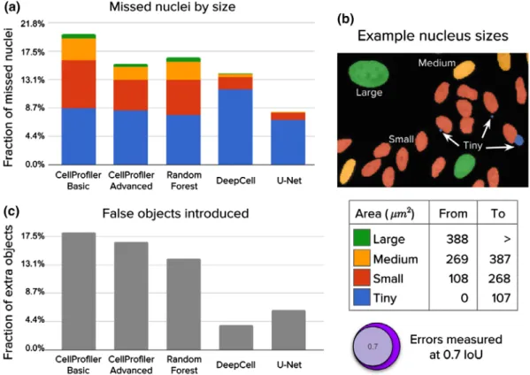
Deep learning methods make fewer segmentation mistakes compared to classical pipelines, effectively correcting most of their typical errors (Figs. 3 and 4). Here, an error is defined as when a nucleus in the ground truth is missed in an esti- mated segmentation mask after applying a minimum IoU threshold of 0.7. By this metric, U-Net achieves an error rate of 8.1%, DeepCell 14.0%, Random Forest 16.5%, advanced CellProfiler 15.5%, and basic CellProfiler 20.1% (Fig. S2).
These results are consistent with the evaluation of accuracy performed at multiple IoU thresholds, indicating that deep learning obtains improved performance.
To understand the performance differences among the evaluated methods, we categorized missed objects by size (Fig. 3a,b) and segmentation errors by type (merges
vs. splits; Fig. 4a,b). An object is missed when the segmen- tation does not meet the minimum IoU threshold crite- rion. A merge is counted when one estimated mask is found covering more than one ground truth mask. Simi- larly, a split is counted when a ground truth mask is being covered by more than one estimated mask. Note that splits and merges are a subset of the total number of errors, and partially overlap with the number of missed objects. That is, some splits and all merges result in one or more miss- ing objects, but not all missing objects are a result of a split or merge.
Deep learning corrects almost all of the errors made by classical pipelines for larger nuclei. We also note that all methods usually fail to capture tiny nuclei correctly (gener- ally, micronuclei, which are readily confounded with debris or artifacts, and represent about 15% of all objects in the test set; Fig. 3a). Interestingly, deep learning tends to accumulate errors for tiny nuclei only, while the CellProfiler pipelines and Random Forests tend to make errors across all sizes (Fig. 3b). Tiny nuclei are missed for several reasons, includ- ing merging with bigger objects, confounding with debris, or failing to preserve enough object signal for the post- processing routines. Some of these issues can be addressed by developing multi-scale segmentation methods or by increasing the resolution of the input images either optically or computationally.
Figure 3. Analysis of segmentation errors (missed and extra objects). The 5,720 nuclei in the test set were used in this analysis. (a) Fraction of missed nuclei by object size (see table). Missed objects in this analysis were counted using anIoUthreshold of 0.7, which offers a good balance between strict nucleus coverage and robustness to noise in ground truth annotations. (b) Example image illustrating sizes of nuclei.
(c) Fraction of extra or false objects introduced by algorithms. [Colorfigure can be viewed at wileyonlinelibrary.com]
Both deep learning approaches are effective at recogniz- ing boundaries to separate touching nuclei and correct typical error modes of classical algorithms: merges and splits (Fig. 4a). Split errors produced by the advanced CellProfiler pipeline reveal a trade-off when configuring the parameters of classical algorithms: in order tofix merges we have to accept some more splits. A similar situation happens with U-Net: it has learned to separate clumped nuclei very effectively because the boundary class has 10 times more weight in the loss function, which at the same time forces the network to make some splits to avoid the cost of missing real boundaries (Fig. 3a,c).
We observe different types of errors produced by the two deep learning models. U-Net detects nuclei of all sizes better than DeepCell (Fig. 3a), but also sees imaginary objects more often (Fig. 3c). Also, U-Net is more sensitive than DeepCell at detecting intra-cell edges, which helps introduce fewer merge errors. However, U-Net also see edges where it should not, leading to more splitting errors as well (Fig. 4a).
Computationally, two main differences between the methods are the use of multiresolution and how spatially coarse feature maps are created. However, we did not investigate the impact on performance of these or other differences (such as filter sizes) in detail in this work.
More Training Data Improves Accuracy and Reduces Errors
We found that training deep learning models with just two images performs already more accurately than an advanced CellProfiler pipeline (Fig. 5a). This is consistent with previous experiments conducted in the DeepCell study (17), demon- strating that the architecture of neural networks can be designed and optimized to perform well in the small data regime. Since training a CNN requires the additional effort of manually annotating example images for learning, limiting the investment of time from expert biologists is valuable.
Data augmentation plays an important role for achieving good generalization results with a small number of images.
DeepCell classifies the center pixel of cell-sized patches, creat- ing a large dataset with thousands of examples obtained from each image. Basic augmentations include image rotations, flips, contrast, and illumination variations. When combined all together, it results in thousands of training points drawn from an image manifold around the available annotated examples. U-Net follows a similar approach but using larger crops and additional data augmentation based on elastic deformations.
Providing more annotated examples improved segmenta- tion accuracy and reduced the number of errors significantly (Fig. 5). Accuracy improves with more data, gaining a few points of performance as more annotated images are used, up to the full 100 images in the training set (Fig. 5a). We found little difference in this trend whether using basic data aug- mentation versus using extra augmentations based on elastic deformations.
Segmentation errors are reduced significantly with more annotated examples, by roughly half (Fig. 5b), but as above, even training with two images produces results better than the advanced CellProfiler baseline. Touching nuclei particu- larly benefit from more training data, which helps to reduce the number of merge errors. As a model learns tofix difficult merge errors by correctly predicting boundaries between touching objects, a trade-off occurs: some split errors appear in ambiguous regions where no boundaries should be predicted. This effect makes the number of split errors increase with more data, albeit at a slower rate and rep- resenting a very small fraction of the total number of errors, while being still fewer than the number of splits made by the advanced CellProfiler pipeline.
Providing a Variety of Training Images Improves Generalization
Preventing overfitting is an important part of training deep learning models. In our study, we followed the best practices, discussed in detail in the DeepCell work, to mitigate the effect of overfitting: (a) collection of a large annotated dataset for Figure 4.Analysis of segmentation errors (splits and merged objects). The 5,720 nuclei in the test set were used in this analysis.
(a) Fraction of merged and split nuclei. These errors are identified by masks that cover multiple objects with at least 0.1IoU. (b) Example merges and splits. [Colorfigure can be viewed at wileyonlinelibrary.com]
training; (b) the use of pixel normalization and batch normal- ization to control data and feature variations, respectively;
(c) the adoption of data augmentation; (d) weight decay to control parameter variations. Besides all these known strate- gies, we also found that including example images with tech- nical variations in the training set (such as experimental noise or the presence of artifacts) can prevent overfitting, serving as an additional source of regularization.
We found that training with images that exhibit different types of noise produces models that transfer better to other sets (Fig. 6a). In contrast, training on an image set that has homogeneous acquisition conditions does not transfer as well to other experiments (Fig. 6b). We tested U-Net models trained on one image set and evaluated their performance when transferring to another set. In one case we took images of nuclei from a prior study (“Van Valen’s Set”)(17), rep- resenting different experiments and including representative examples of diverse signal qualities, cell lines, and acquisition conditions (Fig. 6d). In the other case we used the BBBC039 image collection which exhibits homogeneous signal quality and was acquired under similar technical conditions (Fig. 6c).
A model trained only on the 9 diverse images of Van Valen’s set generalizes well to test images in BBBC039, improving performance over the baseline (Fig. 6a) and reaching comparable performance to the model trained on BBBC039 training images. Note that training a network on images of BBBC039 improves performance with respect to the CellProfiler baseline. The transferred model does notfix all the errors, likely because the number of training examples is limited. Nevertheless, the transferred performance indicates
that it is possible to reuse models across experiments to improve segmentation accuracy.
A transfer from the more homogenous BBBC039 set to the more diverse Van Valen’s set is less successful: a model trained with 100 examples from the BBBC039 set fails to improve on the test set of Van Valen’s images despite the availability of more data (Fig. 6b). This demonstrates the challenges of dealing with varying signal quality, which is a frequent concern in high-throughput and high-content screens. The large gap in performance is explained by varying signal conditions (Fig. 6c,d): because the model did not observe these variations during training, it fails to correctly segment test images.
The CellProfiler pipelines also confirm the difficulty of handling noisy images. A single pipeline cannot deal with all variations in Van Valen’s test set, requiring the adjustment of advanced settings and the splitting of cases into two different pipelines. In BBBC039, a single pipeline works well due in part to the homogeneity of signal in this collection; the errors are due to challenging phenotypic variations, such as tiny nuclei or clumped objects.
Deep Learning Needs More Computing and Annotation Time than Classical Methods
Although we found the performance of deep learning to be favorable in terms of improving segmentation accuracy, we also found that this comes at higher computational cost and annotation time. First, deep learning requires significantly more time to prepare training data with manual annotations (Fig. 7a). Second, deep learning needs the researchers to train Figure 5.Impact of the number of annotated images used for training a U-Net model. Basic augmentations includeflips, 90rotations, and random crops. Extra augmentations include the basic plus elastic deformations. (a) Accuracy improves as a function of the number of training images, up to a plateau around 20 images (representing roughly 2,000 nuclei). (b) Segmentation errors are reduced overall as the number of training images increases, but the impact differs for merges versus splits. The advanced CellProfiler pipeline is shown as dotted lines throughout. Results are reported using the validation set to prevent over-optimizing models in the test set (holdout). For all experiments, we randomly sampled (with replacement) subsets (n= 2, 4, 6, 8, 10, 20, 40, 60, 80, 100) of images from the training set (n= 100) and repeated 10 times to evaluate performance. Data points in plots are the mean of repetitions. Although the percent overlap between the random samples increases with increasing sample size, and is 100% forn= 100, we nonetheless kept the number of repeats fixed (=10) for consistency. The numbers below each arrow indicate the reduction in number of errors for each category of errors. [Color figure can be viewed at wileyonlinelibrary.com]
Figure 6.Signal quality is the main challenge when transferring models across experiments: Performance differences when models are trained and evaluated in different experiments. (a) Models evaluated on the BBBC039 test set, including a U-Net trained on the same set, another U-Net trained on Van Valen’s set, and a CellProfiler pipeline. The results indicate that transferring the model from one screen to another can bring improved performance. (b) Models evaluated in Van Valen’s test set, including CellProfiler baselines adapted to this set, a U-Net trained on the same set, and another U-Net trained on BBBC039. The results illustrate the challenges of dealing with large signal variation. (c) Example images from BBBC039 showing homogeneous signal with uniform background, which is reflected in the aggregated histogram offluorescent intensities for this dataset, with a bimodal distribution and easily separable peaks. (d) Example images from Van Valen’s set illustrating various types of realistic artifacts, such as background noise and high signal variance, also observed in the corresponding histogram with higher density between the peaks of the bimodal distribution. Number of training images:
100 in BBBC039 and 9 in Van Valen. Number of test images: 50 in BBBC039 and 3 in Van Valen. [Color figure can be viewed at wileyonlinelibrary.com]
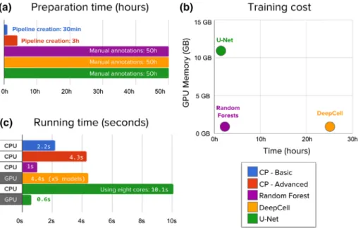
Figure 7.Evaluation of the time needed to create annotations, train, and run segmentation models. (a) Preparation time measures hands on, expert time annotating images or creating CellProfiler pipelines. Manually annotating 100 training images with about 11,500 nuclei requires significantly longer times. (b) Machine learning models need to be trained while CellProfiler pipelines do not need additional processing. Neural network training was run on a single NVIDIA Titan X GPU. DeepCell trains an ensemble offive models, which was used in all evaluations. (c) CellProfiler pipelines and Random Forests are run on new images using CPU cores to measure the computational cost of segmenting a single image. Deep learning needs significantly more resources to accomplish the task, but can be accelerated using GPUs, which have thousands of computing cores that allow algorithms to run operations in parallel. This reduces significantly the elapsed time, making it practical and even faster than classical solutions. [Colorfigure can be viewed at wileyonlinelibrary.com]
a model and tune its parameters (Fig. 7b), usually with special hardware. Third, when a model has been trained, it is slower to run on new images than classical algorithms (Fig. 7c).
However, running times can be accelerated using graphic cards, which makes the technique usable in practice.
We observed that the time invested by experts for anno- tating images is significantly longer than configuring Cel- lProfiler segmentation pipelines (Fig. 7a). We estimate that manually annotating 100 images for training (~11,500 objects) takes 50 h of work using an assisted-segmentation tool. In contrast, a basic CellProfiler pipeline can be calibrated in 15–30 min of interaction with the tool, setting up a config- uration that even users without extensive experience nor computational expertise could complete. CellProfiler is very flexible and allows users to add more modules in order to correct certain errors and factor out artifacts, creating an advanced pipeline that can take from 1 to 3 h.
Training deep learning models takes substantial comput- ing time on GPUs, while CellProfiler pipelines do not need any additional training or postprocessing (Fig. 7b). In our study, the deep learning models under evaluation are big enough to need a GPU for training, but light enough to be trained in a few hours. In particular, a U-Net can be trained in a single NVIDIA Titan X GPU in just 1 h, while DeepCell takes 25 h for an ensemble offive networks (as suggested in the original work (17)). Also, training models may need pre- liminary experiments to calibrate hyperparameters of the neu- ral network (e.g., learning rate, batch size, epochs), which adds more hands-on time.
Notice the trade-off between memory and training time of deep learning models. DeepCell trains a compact neural network with small memory requirements, which makes it ideal for running experiments efficiently in modest hardware configurations. This design has the additional advantage of allowing strategic pixel sampling for training, resulting in a balanced selection of pixels from the background, boundary, and interior of cells. In contrast, U-Net trains larger neural network models that process all the pixels simultaneously using a fully convolutional approach resulting in high mem- ory requirements and, therefore, needing expensive GPU hardware for training. This can be constraining for laborato- ries not equipped to run computationally heavy experiments.
When segmenting new images using CPU cores, deep learning models are slower than CellProfiler pipelines (Fig. 7c). The computational complexity in terms of space (memory) and time (operations) of a CNN is proportional to the number of layers, the number of filters, and the size of images. As these architectures get deeper and more com- plex, they involve more operations to produce the final result, and thus require more computing power. This is in contrast to classical segmentation algorithms whose thresholding andfiltering operations have relatively limited computing requirements that scale well with the size of images. Even with 8 times more cores, a U-Net takes 10.1 s to segment a single image, which results in about 20 times more computing power requirements than the advanced CellProfiler pipeline. CellProfiler pipelines are run in a single
CPU core and take 2.2 and 4.3 s for the basic and advanced pipelines respectively.
Using GPU acceleration can significantly speed up the computations of deep learning models, making them very usable and efficient in practice (Fig. 7c). Segmenting a single image with a U-Net model takes only 0.6 s on a Nvidia Titan X GPU, improving computation times by a factor of 16×.
Note that no batching was used for prediction, which can accelerate computation of groups of images even further. In our experiments, a single DeepCell network ran at 4.4 s per image with GPU acceleration, which has been sped up using a custom implementation of dilated convolution and pooling operations in Theano. Even faster versions of these operations are available in modern deep learning frameworks, such as TensorFlow. These results show that deep learning models are faster than classical algorithms when using appropriate hardware and efficient implementations.
Better Segmentations Improve High-Content Cytometry Screens
Accurate nucleus segmentation improves the sensitivity of cytometry screens in real world high-throughput applications.
To quantify this effect, we evaluated the performance of the segmentation using the Z’-factor in a high-content experi- ment. The goal of this experiment is to identify compounds that disrupt normal cell cycle, thus, we measured the DNA content of single cells using the total integrated intensity within each segmented nucleus as a readout.
We selected a subset of 10 compounds screened with high-replicates in the BBBC022 image collection (Fig. S3) to measure their effect to the cell cycle compared to DMSO treated wells (negative controls). For each image, we mea- sured the integrated intensity of nuclei and estimated the pro- portion of cells with 4N DNA content. After controlling for potential batch effects, we observed that none of the com- pounds yield a sufficiently high Z’-factor that indicates cell cycle disruption. It should be noted that the compounds selected are not known to have effects on the cell cycle—thus, we did not expect them all to yield a detectable phenotype in this assay. However, the measurements were a good choice for our purposes, because we wanted a nucleus-based readout whose baseline quality was not so high so as to leave no room for improvement with better segmentation. For 7 out of the 10 selected compounds we observed improved Z’-factor scores when the segmentation was carried out with a deep learning model, indicating more sensitivity of the screen for detecting interesting compounds.
Other studies have also observed improved assay quality when using deep learning for cell segmentation. For instance, analyzing the structure of tumors in tissues using multiplexed ion beam imaging reveals the spatial organization and response of immune cells in cancer patients (50). These results were obtained with a computational workflow powered by the DeepCell library, demonstrating that deep learning can accurately segment single cells in challenging imaging conditions.
D
ISCUSSIONPrevious studies of cell segmentation observed minor improvements when comparing deep learning methods versus classical algorithms using the Jaccard index (17). Also, a recent cell tracking challenge analysis noted that thresholding approaches are still the top solutions for segmenting cells (19); their ranking score is also the Jaccard index. We argue that these evaluation methods do not satisfactorily capture biologically important error modes, making it difficult to appropriately assess cell and nuclei segmentation algorithms.
We presented an evaluation framework focused on object level accuracy, which captures biological interpretations more naturally than pixel-level scores (Fig. S1).
The objects of interest in biology are full instances of nuclei that experts can identify by eye. Our results show that deep learning strategies improve segmentation accuracy and reduce the number of errors significantly as compared to base- lines based on classical image processing and machine learning.
However, we show that these methods still make mistakes that experts do not. Being able to quantify these mistakes explicitly will drive future research toward better methods that could match human performance. In our benchmark, deep learning provided improved performance in all the tests that measured accuracy and error rates. Despite requiring significant annota- tion effort and computational cost, deep learning methods can have a positive impact on the quality and reliability of the mea- surements extracted fromfluorescence images.
Improved Accuracy
The proposed evaluation metrics are able to distinguish bio- logically meaningful errors, helping to better differentiate the performance of segmentation models. The results of our benchmark show that deep learning methods can bring signif- icant advantages for segmenting single objects in new images, compared to manually configured image processing algo- rithms and classic machine learning. Both DeepCell and U-Net are able to improve the segmentation accuracy (Figs. 2 and S1) and reduce the total number of errors (Figs. 3–4, and S2). This shows that even though these models were created for generic cell segmentation and optimized for learning from small datasets, they can be trained to successfully identify nuclei using large sets of images.
The analysis of errors indicates that deep learning canfix most of the segmentation errors observed in classical algo- rithms, especially merges. One special type of error that repre- sents a challenge for both deep learning models is the segmentation of tiny nuclei (micronuclei and other debris, if of interest in an experiment). In extensive experiments conducted in the DeepCell study (17), the size of the receptivefield has been shown to be a key parameter to improve performance, suggesting that crops that fully cover single cells are sufficiently informative for accurate segmentation. Increasing the resolu- tion of images, either during acquisition (51) or with computa- tional methods such as resizing images to make objects look bigger, may helpfix these errors. Alternatively, different loss functions adapted to this problem might be designed.
Training Data
In our evaluation, the amount of training data was shown to be an important factor to reduce the number of errors. Our results confirm that training a neural network with only a few images is enough to get improved performance relative to nondeep learning baselines. However, in order to improve accuracy and leverage the learning capacity of deep learning models, more data is required. Importantly, a neural network can also be reused across experiments, as long as the training data incorporates variations in morphological phenotypes as well as variations in signal quality and acquisition conditions.
Datasets used for training supervised machine learning models are prone to contain human errors and subjective biases. Errors include accidentally overlooking real objects, and biases include differences in opinion about precise boundaries.
We used multiple annotators for practical reasons and also to reflect real differences of opinion among biologists. When mul- tiple annotators are used, it is recommended to agree upon best practices to minimize errors and curate useful ground truth. A useful dataset is one that has enough examples of varied situa- tions and where the real signal is not dominated by subjective noise. We believe our dataset is such a resource, where biolo- gists agreed on covering all possible nuclei phenotypes and worked hard to be as consistent as possible, while allowing for individual variation that might arise from subjectivity or even screen brightness during annotation. Although assigning two or more annotators to the same image can create a very high- quality dataset, given the amount of inherent subjectivity among annotators, we decided it would be more useful to have twice the amount of good-quality ground truth with a single annotator per image. Future efforts tofix existing issues and to expand the dataset would be welcome.
We argue that a single deep learning model might be con- structed to address all the challenges of nucleus segmentation in fluorescence images if a diverse database of annotated examples were to be collected to incorporate these two critical axes of var- iation. We advocate for collecting that data collaboratively from different research labs, so everyone will benefit from a shared resource that can be used for training robust neural networks.
We have begun such an effort via the 2018 Data Science Bowl https://www.kaggle.com/c/data-science-bowl-2018/.
Computational Cost
Deep learning models generally run a higher computational cost. GPUs can be useful in microscopy laboratories for accel- erating accurate neural network models; if acquisition or maintenance is prohibitive, cloud computing allows laborato- ries to run deep learning models using remote computing resources on demand. Adopting these solutions will equip biologists with essential tools for many other image analysis tasks based on artificial intelligence in the future.
A
CKNOWLEDGMENTThe authors thank Beth Cimini and Minh Doan for their efforts and guidance when annotating the image set used for this research. The authors also thank Mohammad Rohban and Beth Cimini for fruitful discussions and key insights to design
experiments and write the manuscript. The authors are grateful to David Van Valen for his help while running the DeepCell library and for his constructive suggestions to improve the clar- ity of the manuscript. Funding was provided by the National Institute of General Medical Sciences of the National Institutes of Health under MIRA award number R35 GM122547 (to AEC). The experiments were run on GPUs donated by NVIDIA Corporation through their GPU Grant Program (to AEC). C.M. acknowledges support from the HAS- LENDULET-BIOMAG and from the European Union and the European Regional Development Funds GINOP-2.3.2-15- 2016-00006.
A
UTHORC
ONTRIBUTIONSJCC contributed experiments, data analysis, software develop- ment, and manuscript writing. JR contributed experiments, data preparation, data analysis, and software development.
AG contributed experimental design, data preparation, and software development. TB contributed experiments, software development, and manuscript writing. KWK contributed experiments, data preparation, and data analysis. MB contrib- uted experiments and data analysis. MC contributed experi- ments. CM contributed data preparation and software development. SS contributed experimental design and manu- script writing. FT contributed experimental design and manu- script writing. AEC contributed experimental design, data interpretation, and manuscript writing.
R
EFERENCES1. Boutros M, Heigwer F, Laufer C. Microscopy-based high-content screening. Cell 2015;163:1314–1325.
2. Mattiazzi Usaj M, Styles EB, Verster AJ, Friesen H, Boone C, Andrews BJ. High- content screening for quantitative cell biology. Trends Cell Biol 2016;26(8):598–611.
3. Caicedo JC, Singh S, Carpenter AE. Applications in image-based profiling of pertur- bations. Curr Opin Biotechnol 2016;39:134–142.
4. Bougen-Zhukov N, Loh SY, Lee HK, Loo L-H. Large-scale image-based screening and profiling of cellular phenotypes. Cytometry A 2016. http://dx.doi.org/10.1002/- cyto.a.22909;91:115–125.
5. Williams E, Moore J, Li SW, Rustici G, Tarkowska A, Chessel A, Leo S, Antal B, Ferguson RK, Sarkans U, et al. The image data resource: A bioimage data integra- tion and publication platform. Nat Methods 2017;14:775–781.
6. Meijering E. Cell segmentation: 50 years down the road [life sciences]. IEEE Signal Process Mag 2012;29:140–145.
7. Otsu N. A threshold selection method from gray-level histograms. IEEE Trans Syst Man Cybern 1979;9:62–66.
8. Beucher S, Lantuejoul C. Use of watersheds in contour detection. In: Proceedings of the International Workshop on Image Processing; 1979. https://ci.nii.ac.jp/naid/
10008961959/.
9. Wählby C, Sintorn I-M, Erlandsson F, Borgefors G, Bengtsson E. Combining inten- sity, edge and shape information for 2D and 3D segmentation of cell nuclei in tissue sections. J Microsc 2004;215:67–76.
10. Sommer C, Straehle C, Köthe U, Hamprecht FA. Ilastik: Interactive learning and segmentation toolkit. In: IEEE International Symposium on Biomedical Imaging:
From Nano to Macro. ieeexploreieeeorg; 2011. pp 230–233.
11. Eliceiri KW, Berthold MR, Goldberg IG, Ibáñez L, Manjunath BS, Martone ME, Murphy RF, Peng H, Plant AL, Roysam B, et al. Biological imaging software tools.
Nat Methods 2012;9:697–710.
12. Carpenter AE, Jones TR, Lamprecht MR, Clarke C, Kang IH, Friman O, Guertin DA, Chang JH, Lindquist RA, Moffat J, et al. CellProfiler: Image analysis software for identifying and quantifying cell phenotypes. Genome Biol 2006;7:R100.
13. Schindelin J, Arganda-Carreras I, Frise E, Kaynig V, Longair M, Pietzsch T, Preibisch S, Rueden C, Saalfeld S, Schmid B, et al. Fiji: An open-source platform for biological-image analysis. Nat Methods 2012;9:676–682.
14. LeCun Y, Bengio Y, Hinton G. Deep learning. Nature 2015;521:436–444.
15. Mnih V, Kavukcuoglu K, Silver D, Rusu AA, Veness J, Bellemare MG, Graves A, Riedmiller M, Fidjeland AK, Ostrovski G, et al. Human-level control through deep reinforcement learning. Nature 2015;518:529–533.
16. Ronneberger O, Fischer P, Brox T. U-net: Convolutional networks for biomedical image segmentation. Med Image Comput Comput Assist Interv 2015;9351:234–241.
http://link.springer.com/chapter/10.1007/978-3-319-24574-4_28.
17. Van Valen DA, Kudo T, Lane KM, Macklin DN, Quach NT, DeFelice MM, Maayan I, Tanouchi Y, Ashley EA, Covert MW. Deep learning automates the quan- titative analysis of individual cells in live-cell imaging experiments. PLoS Comput Biol 2016;12:e1005177.
18. Dima AA, Elliott JT, Filliben JJ, Halter M, Peskin A, Bernal J, Kociolek M, Brady MC, Tang HC, Plant AL. Comparison of segmentation algorithms forfluores- cence microscopy images of cells. Cytometry A 2011;79:545–559.
19. Ulman V, Maška M, Magnusson KEG, Ronneberger O, Haubold C, Harder N, Matula P, Matula P, Svoboda D, Radojevic M, et al. An objective comparison of cell-tracking algorithms. Nat Methods 2017;14:1141–1152.
20. Rapoport DH, Becker T, Madany Mamlouk A, Schicktanz S, Kruse C. A novel vali- dation algorithm allows for automated cell tracking and the extraction of biologi- cally meaningful parameters. PLoS One 2011;6:e27315.
21. Wienert S, Heim D, Saeger K, Stenzinger A, Beil M, Hufnagl P, Dietel M, Denkert C, Klauschen F. Detection and segmentation of cell nuclei in virtual microscopy images: A minimum-model approach. Sci Rep 2012;2:503.
22. Gustafsdottir SM, Ljosa V, Sokolnicki KL, Anthony Wilson J, Walpita D, Kemp MM, Petri Seiler K, Carrel HA, Golub TR, Schreiber SL, et al. Multiplex cyto- logical profiling assay to measure diverse cellular states. PLoS One 2013;8:e80999.
23. Bray M-A, Singh S, Han H, Davis CT, Borgeson B, Hartland C, Kost-Alimova M, Gustafsdottir SM, Gibson CC, Carpenter AE. Cell Painting. A high-content image- based assay for morphological profiling using multiplexedfluorescent dyes. bioRxiv 2016;049817. 2016. http://biorxiv.org/content/early/2016/04/28/049817.
24. Fenech M, Morley AA. Measurement of micronuclei in lymphocytes. Mutat Res 1985;147:29–36.
25. Norppa H, GC-M F. What do human micronuclei contain? Mutagenesis 2003;18:
221–233.
26. Zhang C-Z, Spektor A, Cornils H, Francis JM, Jackson EK, Liu S, Meyerson M, Pellman D.
Chromothripsis from DNA damage in micronuclei. Nature 2015;522:179–184.
27. Harding SM, Benci JL, Irianto J, Discher DE, Minn AJ, Greenberg RA. Mitotic pro- gression following DNA damage enables pattern recognition within micronuclei.
Nature 2017;548:466–470.
28. Ly P, Teitz LS, Kim DH, Shoshani O, Skaletsky H, Fachinetti D, Page DC, Cleveland DW. Selective Y centromere inactivation triggers chromosome shattering in micronuclei and repair by non-homologous end joining. Nat Cell Biol 2017;19:68–75.
29. Hintzsche H, Hemmann U, Poth A, Utesch D, Lott J, Stopper H. Working group“in vitro micronucleus test”, Gesellschaft für Umwelt-Mutationsforschung (GUM, German- speaking section of the European environmental mutagenesis and genomics society EEMGS). Fate of micronuclei and micronucleated cells. Mutat Res 2017;771:85–98.
30. Hughes AJ, Mornin JD, Biswas SK, Beck LE, Bauer DP, Raj A, Bianco S, Gartner ZJ.
Quanti.Us: A tool for rapid, flexible, crowd-based annotation of images. Nat Methods 2018;15:587–590.
31. Hariharan B, Arbeláez P, Girshick R, Malik J.. Simultaneous detection and segmen- tation. arXiv [Cs.CV]. 2014. http://arxiv.org/abs/1407.1808.
32. Shelhamer E, Long J, Darrell T. Fully convolutional networks for semantic segmen- tation. arXiv [Cs.CV]. 2016. http://arxiv.org/abs/1605.06211.
33. Fiorio C, Gustedt J. Two linear time union-find strategies for image processing.
Theor Comput Sci 1996;154:165–181.
34. Chen S, Haralick RM. Recursive erosion, dilation, opening, and closing transforms.
IEEE Trans Image Process 1995;4:335–345.
35. He K, Gkioxari G, Dollár P, Girshick R. Mask R-CNN. In: IEEE International Con- ference on Computer Vision (ICCV); 2017. pp 2980–2988.
36. Zoph B, Le QV. Neural architecture search with reinforcement learning. arXiv [Cs.LG]; 2016. http://arxiv.org/abs/1611.01578.
37. Bannon D, Moen E, Borba E, Ho A, Camplisson I, Chang B, Osterman E, Graf W, Van Valen D. DeepCell 2.0: Automated cloud deployment of deep learning models for large-scale cellular image analysis. bioRxiv; 2018. 505032. https://www.biorxiv.
org/content/early/2018/12/22/505032.
38. Nair V, Hinton GE. Rectified linear units improve restricted boltzmann machines.
In: Proceedings of the 27th international conference on machine learning (ICML- 10). cs.toronto.edu; 2010. pp 807–814.
39. Ioffe S, Szegedy C. Batch normalization: Accelerating deep network training by reducing internal covariate shift. In: International Conference on Machine Learning.
jmlr.org; 2015. pp 448–456.
40. Hinton GE, Salakhutdinov RR. Reducing the dimensionality of data with neural net- works. Science 2006;313:504–507.
41. McQuin C, Goodman A, Chernyshev V, Kamentsky L, Cimini BA, Karhohs KW, Doan M, Ding L, Rafelski SM, Thirstrup D, et al. CellProfiler 3.0: Next generation image processing for biology. PLoS Comput Biol 2018. https://doi.org/10.1371/
journal.pbio.2005970.
42. Falk T, Mai D, Bensch R, Çiçek Ö, Abdulkadir A, Marrakchi Y, Böhm A, Deubner J, Jäckel Z, Seiwald K, et al. U-net: Deep learning for cell counting, detec- tion, and morphometry. Nat Methods 2018;16:67–70. https://doi.org/10.1038/
s41592-018-0261-2.
43. Gudla PR, Nandy K, Collins J, Meaburn KJ, Misteli T, Lockett SJ. A high- throughput system for segmenting nuclei using multiscale techniques. Cytometry A 2008;73:451–466.
44. Singh S, Raman S, Rittscher J, Machiraju R. Segmentation evaluation forfluores- cence microscopy images of biological objects. In: MIAAB 2009 International Work- shop Proceedings. Academia.Edu; 2009. pp 1–5.
45. Everingham M, Van Gool L, Williams CKI, Winn J, Zisserman A. The Pascal visual object classes (VOC) challenge. Int J Comput Vis 2010;88:303–338.