Measurement-driven Large Eddy Simulation of dispersion in street canyons of variable building height
B alint Papp
a,*, Gergely Krist of
a, Bal azs Ist ok
a, M arton Koren
a, M arton Balcz o
a, Mikl os Balogh
aaDepartment of Fluid Mechanics, Faculty of Mechanical Engineering, Budapest University of Technology and Economics, M}uegyetem rkp. 3, 1111, Budapest, Hungary
A R T I C L E I N F O Keywords:
Urban air quality Dispersion of aerosols Wind tunnel experiment Large Eddy Simulation (LES) Variable building height Street canyons Periodic domain
Transient Wind Forcing (TWF) Traffic-induced air pollution Lagrangian dispersion model
A B S T R A C T
The ventilation efficiency of three periodic building patterns of equal total volume and packing density is investigated: street canyons bounded byHuniform and 0.5H/1.5Hvariable height buildings, via wind tunnel measurements and Large Eddy Simulation. The numerical model utilizes the Transient Wind Forcing method to take the effect of eddies larger than the domain size into account, and a special Lagrangian dispersion model, which allows for the calculation of particle trajectories exceeding the periodic boundaries of the LES domain. The spatial and temporal characteristics of the concentration responses of both pulse-like and steady point sources located at the street surfaces are analyzed. It is shown that the variable building height has a favorable effect on urban ventilation in densely built areas: the average near-ground concentration can be reduced by up to 70% for the variable height buildings in a staggered arrangement. In terms of velocity, turbulence and concentration distributions, the model results are consistent with the experiments, verifying the applicability of the model for comparative air quality studies. Since the presented dispersion model is capable of handling dynamic changes in wind direction and magnitude, the accuracy of the TWF model can potentially overcome the limitations of wind tunnel tests.
1. Introduction
As urbanization advances, access to healthy air is becoming increas- ingly important in the lives of city dwellers. The individuals’exposure to traffic-related air pollutants and airborne pathogens is increasing due to the declining dilution associated with the concentration of pollutant sources. There are some feasible technical measures to limit transmission and promote ventilation, the effectiveness of which can be assessed by experimental or numerical simulation methods. The results of field measurements, wind tunnel tests, and microscale meteorological models are strongly related to the examined geometry as well as to the flow characteristics of the atmospheric boundary layer, which are also ge- ometry dependent. The results are, therefore, difficult to generalize.
Periodically repeated patterns, such as building blocks or junctions, are key features of the urban canopy. By exploiting the periodicity, the number of model parameters can be significantly reduced, facilitating the generalization of the model results. Consequently, repetitive geometric patterns are preferred subjects of field experiments (Biltolft, 2001;
Kanda, 2009;Chen et al., 2020), wind tunnel measurements (Leitl et al., 2007; Yee and Blitolft, 2004) and numerical models (Eichhorn and Balczo, 2008;Santiago et al., 2010;Dejoan et al., 2010;Rakai and Kristof,
2010). For the latter, the repetitive surface patterns can be easily con- structed by applying periodic boundary conditions at the lateral sides of the simulation domain, thus taking into account an infinitely large re- petitive structure in a small modeling box. A further advantage of this method is that it does not require the exact definition of inlet boundary conditions, which is particularly beneficial for CFD models utilizing Large Eddy Simulation (LES)–a turbulence model that can produce more accurate results in urbanflow and dispersion compared to the conven- tional RANS approaches (Tominaga and Stathopoulos, 2011;Tominaga et al., 2013). The inlet boundary conditions for LES may be defined ac- cording to the method proposed byKataoka and Mizuno (2002); alter- natively, the method proposed byXie and Castro (2008)andXie (2011) using velocity time series fromfield observations supplemented with artificially generated turbulence. Nevertheless, the inlet boundary con- ditions introduce additional model parameters and modeling un- certainties into the analysis. Instead of prescribing the inlet velocity and turbulence profiles, in the periodic models, theflow can be created by a spatially distributed driving force, the volume integral of which balances the drag force of the surface objects, such as buildings and vegetation.
Most periodic models are driven by a constant intensity volumetric driving force (Ciofalo, 1996;Su et al., 1998;Cheng et al., 2003;Baker
* Corresponding author.
E-mail address:papp@ara.bme.hu(B. Papp).
Contents lists available atScienceDirect
Journal of Wind Engineering & Industrial Aerodynamics
journal homepage:www.elsevier.com/locate/jweia
https://doi.org/10.1016/j.jweia.2020.104495
Received 31 August 2020; Received in revised form 2 December 2020; Accepted 20 December 2020 Available online xxxx
0167-6105/©2020 The Authors. Published by Elsevier Ltd. This is an open access article under the CC BY license (http://creativecommons.org/licenses/by/4.0/).
Journal of Wind Engineering & Industrial Aerodynamics 210 (2021) 104495
et al., 2004;Cai et al., 2008;Letzel et al., 2008;Kikumoto and Ooka, 2012;Kristof and Füle, 2017) which requires the specification of only two model parameters: the horizontal components of the pressure gradient. The disadvantage of the static pressure gradient-driven LES models is the fact that the size of the resolved turbulent structures is limited by the size of the computational domain, which also limits the accuracy of dispersion results since the larger turbulent structures have a substantial contribution to the transport processes. The literature review byTominaga and Stathopoulos (2016)also encourages the investigation of the influence of the atmospheric turbulence scales on dispersion.
The above-described problem can be solved by using a transient driving force (Kristof et al., 2020). Measurement data or the results of larger-scale meteorological models can be used to control the driving force in a way that the horizontal components of the calculated velocity follow the prescribed wind speed at a designated observation point.
An essential element of the Transient Wind Forcing model presented in our previous study (Kristof et al., 2020) is that the turbulent spectrum is divided into microscopic, mesoscopic, and macroscopic parts based on the size of the smallest and largest turbulent structures that can be resolved in the model. The microscopic turbulence is considered using a Subgrid-Scale Stress (SGS) model; the LES model resolves the mesoscopic turbulence, so it appears in the results in the form of velocityfluctuations over time. Furthermore, the effect of macroscopic turbulence is taken into account by the transient driving force, so the frequency of the pro- pulsion must match the lowest frequency of the mesoscopic turbulence.
The relaxation time of the propulsion control (Δt0) must be chosen in proportion to the ratio of the domain length and the average wind speed measured at the reference point. The temporal resolution of the measured data set must befiner than the relaxation time of the force control.
At the time of publishing the TWF model, the authors were not aware of the Real-Time Boundary wind Condition (RTBC) model previously published byZhang et al. (2011), which was, to our present knowledge, the earliest measurement-driven periodic LES model. Comparing the two methods, a significant difference is that the RTBC model does notfit the time parameter of the propulsion to the turbulence time scale resolved in the model; moreover, the resolution of the measurement data set is well below the control’s cut-off frequency, which resulted in a series of steady flows. The most recent version of the RTBC model (Li et al., 2020) is more elaborate in this regard, due tofitting the time parameter of the method to the frequency corresponding to the peak of the pre-multiplied pow- er-spectrum of the measured turbulence.
There is also a crucial difference in the choice of the location of the gauging point: in the case of the RTBC model, the observation point is located near the roof of the buildings (z/H¼1.1), so the gauge inter- mittently fell in the wake of the building; consequently, the driving wind speed does not adequately represent the wind speed above the urban canopy. Presumably, this caused the simulation to produce windless episodes often. The spatial distribution of the driving force is homoge- neous horizontally for both the RTBC and the TWF models, and it follows a prescribed vertical profile. Using a driving force with a Gaussian pro- file, the TWF model produced average velocity and turbulence distribu- tions in street canyons with a height-to-width ratio ofH/W¼2 and 3 that showed good agreement with nearly full-scale measurement data. The RTBC model uses a power-law distribution for the driving force in the vertical direction, which assumption is not yet validated.
In the time-dependent flow field created by the TWF model, the dispersion process is investigated by the Lagrange model, i.e., by deter- mining the trajectories of particles. We track the position of massless par- ticles within the domain and record the number of their streamwise and lateral periodic jumps, which can be used to calculate the position of the particles in a horizontally unlimited space. This method makes it possible to generalize the results of periodic dispersion models to an aperiodic dispersion process, such as the transmission of contaminants from a source canyon to subsequent downstream street canyons. Our previous study (Kristof et al., 2020) has proven that including the large-scale velocity fluctuations in the simulation–instead of working only with the mean wind
characteristics–can significantly influence the resultant pollutant distri- bution, namely, a wider plume and a significant temporal variation of the pollutant concentration in the source canyon was observed. Similar results were shown previously byXie (2011): when including 30 s resolution mesoscale wind data to the street-scale LES simulations, the predicted dispersion was in significantly better agreement with thefield measure- ments than when steady wind conditions were applied.
Previous street canyon models usually employ lengthwise line sources of constant intensity (Meroney et al., 1996;Chan et al., 2002;Simo€ens and Wallace, 2008;Gromke et al., 2016), which represent the steady emission at the traffic lanes. The emission intensity distribution of a spatially inhomogeneous line source, however, can be composed as the sum of the intensity of its sub-surfaces represented by point sources. A similar summation can be performed in time: the changing source in- tensity can be represented by the sum of intermittently active sources of various strengths.
To generalize the results, we analyze the effect of point sources, thus allowing for the investigation of spatially and temporally inhomogeneous emissions, such as exhaust gases leaving a multi-story car park, or even aerosolized pathogens exiting the human respiratory system. The advantage of the Lagrange method is that any number of point sources can be modeled simultaneously because the emission point of each par- ticle is known, thus the effect of different source locations can be distinguished. Also, in wind tunnel models with heterogeneous roof height, it is necessary to test several point sources located along the street, in accordance with the geometrical changes.
The transmission between a source and an observation point is characterized by the local dose distribution, determined by the total residence time of the particles per unit volume. The dose distribution does not depend–in terms of the ensemble mean–on the duration of the emission, only on the total mass of the pollutants emitted, provided that the observation time is long enough to include the entire concentration wave (rise, plateau, and decay; seeFig. 1) caused by the emission. The resulting dose distributions can be used to evaluate the effect of either steady or pulse-like sources. For the latter, a representative concentration response can be determined by averaging the concentration waves generated by several gas-puffs.
For the validation of the numerical model, wind tunnel experiments were performed in the framework of this research, investigating theflow
Fig. 1.Concentration response types and averaging schemes (ensemble and time average) for different kinds of pollutant emissions. The dose response is defined as the integral of all the concentration as the function of time.
and dispersion processes in various parallel street canyon series subjected to perpendicular wind relative to their length axis. The recorded time- resolved two-component LDA data was also used for driving the TWF model. Based on the experimental results, we quantitatively evaluate the accuracy of the numerical model in terms of mean velocity, turbulence quantities, and average concentration distribution of tracer gas emitted from steady point sources of different locations.
The heterogeneity of the building height strongly influences the ventilation of street canyons by modifying the roof-levelflow structures and mixing processes. The wind tunnel measurements ofPascheke et al.
(2008)and the LES simulations ofBoppana et al. (2010)showed that around staggered roughness elements of varying height (0.28H…1.72H in multiple steps) the turbulence intensity was higher, and canopy average concentration (up toH) was lower than for a uniform block height. Based on field experiments, Kanda and Moriizumi (2009) concluded that for not too sparsely located buildings of two block heights (H1andH2), the mass transfer coefficient characterizing the ventilation
of the building arrangement can be approximated by the mass transfer coefficient of an array of uniform homogeneous building heights equal to the difference between the aforementioned block heights (H1–H2).
Nosek et al. (2016,2017)investigated theflow and dispersion pro- cesses in a network of street canyons representative for European inner cities with both uniform and heterogeneous roof heights. The wind tunnel experiments revealed that the building non-uniformity can improve the pollutant removal capability of complex building arrange- ments as well, in the case of numerous wind directions. The favorable effects of building height variability were also observed for typical metropolitan building configurations as well: strictly arranged high-rise buildings of different heights showed enhanced pollutant removing ca- pabilities, seeHang et al. (2012),Chen et al. (2017)and the references therein.
As the building height heterogeneity may be a practical planning concept to improve urban ventilation since it does not adversely affect the economic parameters, the building volume per unit area, the building Fig. 2. (a) Wind tunnel setup with the baffle (1), the building models (2), and the probe traversing system (3). Periodic tower configurations: matrix (b) and staggered arrangement (a, c).
Fig. 3. Plan view of the three investigated building arrangements. Taller buildings are displayed with darker colors. The position of the left and right pollutant sources are indicated by circles. The dashed lines designate the border of the CFD domains of the corresponding cases. Velocity time series were recorded for driving the TWF model over the streamwise left source at 2Hheight. (For interpretation of the references to color in thisfigure legend, the reader is referred to the Web version of this article.)
packing density and the installation raster area are kept constant in our investigations (following Kristof and Füle, 2017). In this paper, we analyze the dose responses to street level pollutant emissions in long, parallel street canyons of constant and variable building height, using numerical models and wind tunnel experiments.
2. Materials and methods 2.1. Wind tunnel measurements
Wind tunnel experiments were performed to investigate theflow and dispersion characteristics of three periodic building arrangements using the closed-circuit horizontal (G€ottingen-type) wind tunnel of the Karman Wind Tunnel Laboratory of the Department of Fluid Mechanics at the Budapest University of Technology and Economics. The wind tunnel has a circular cross-section of 2.6 m diameter at the open test section of 3.8 m length.
2.1.1. Wind tunnel setup and building patterns
For the wind tunnel measurements, three periodically repeated building configurations were constructed from styrofoam. The baseline case consisted of 23 small-scale (M¼1:200), 1/1 (height-to-width,H/W) aspect ratiouniform street canyons, positioned perpendicular to the wind direction. The canyons were constructed using buildings of constantB H¼100 mm100 mm (breadth by height) rectangular cross-section, placed atW¼100 mm distance one after another; hence, the offset be- tween two adjacent streets isS¼200 mm. The 22 canyons–the length of which exceeded the width of the measurement section–are numbered from10 toþ11 in the streamwise direction, with tracer gas sources located in the 0th canyon.
In order to assess the effect of the heterogeneity of the buildings on air quality, two more building arrangements were designed. Towers were constructed by elevating and lowering the rooftops in the middle section of 1.25 m width, in 6 segments by 0.5H. Hence, in each row, three taller and three shorter segments were created, each ofBT¼100 mm 208.33 mm plan area, seeFig. 2andFig. 3. In thematrix arrangement, the tall towers are located behind another tall tower in streamwise (x) di- rection; therefore, the roof height is varying only in the lateral (y) di- rection. Finally, in thestaggered arrangement, the tall towers are shifted laterally relative to the previous and following rows, i.e., the heteroge- neity of the roof height is present in bothxandydirections. Note that all three building configurations have identical total volume.
The building models were subjected to a uniform approachflow. 4.75H upstream of the test section, a 0.6Htall baffle was placed (seeFig. 2), in order to reduce the size of the separation bubble forming over thefirst few rows of buildings. It was found that after the so-called 0th canyon (physi- cally the 11th in streamwise direction), theflow can be considered periodic.
Two identical tracer gas sources of 28 mm diameter wereflush-mounted in the base plate of the building models. As shown inFig. 3, the sources are located in the middle of the 0th canyon in streamwise direction (x¼0) and with a lateral offset of half a tower width (y/T¼ 0.5).
2.1.2. Velocity measurements
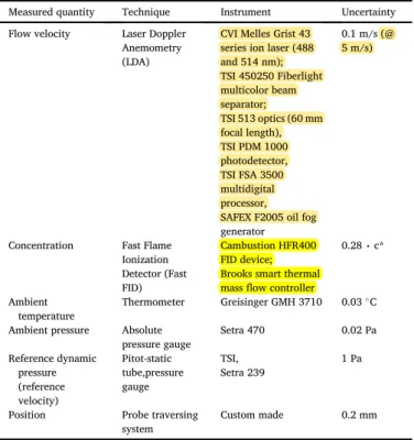
The distribution of the horizontal velocity components for each building pattern was measured using two-component Laser Doppler Anemometry in the 0th and 4th canyons. The complete measurement instrumentation is listed inTable 1. The optics of the LDA device was mounted on the probe traversing system of the wind tunnel to enable precise and repeatable positioning. The system incorporates Bragg-cells for both velocity components, so the sign of the velocity components could be identified. The pass-through time of each particle signal was recorded and further used as weights when calculating the average ve- locity (gate-time weighting).
The velocity measurement in each gauging point took 150 s with a sampling frequency range of 100…1000þHz (depending on how effi- ciently the seeding is able to access the gauging points), resulting in time Table 1
Measurement instrumentation.
Measured quantity Technique Instrument Uncertainty
Flow velocity Laser Doppler Anemometry (LDA)
CVI Melles Grist 43 series ion laser (488 and 514 nm);
TSI 450250 Fiberlight multicolor beam separator;
TSI 513 optics (60 mm focal length), TSI PDM 1000 photodetector, TSI FSA 3500 multidigital processor, SAFEX F2005 oil fog generator
0.1 m/s (@
5 m/s)
Concentration Fast Flame Ionization Detector (Fast FID)
Cambustion HFR400 FID device;
Brooks smart thermal massflow controller
0.28∙c*
Ambient temperature
Thermometer Greisinger GMH 3710 0.03C Ambient pressure Absolute
pressure gauge
Setra 470 0.02 Pa
Reference dynamic pressure (reference velocity)
Pitot-static tube,pressure gauge
TSI, Setra 239
1 Pa
Position Probe traversing
system
Custom made 0.2 mm
Fig. 4.Left: dependence of the mean velocity results on the Reynolds number. Right: dependence of the mean velocity profiles on the streamwise position. UC:
uniform canyons, MT: matrix towers, ST: staggered towers.
statistics of the horizontal velocity components with less than 5% sta- tistical uncertainty in the streamwise direction, except for the points with extremely large turbulence intensity values. In the reference points, the representativeness uncertainty values are 0.57% for the uniform can- yons, 0.56% for the matrix towers, and 1.06% for the staggered towers.
The representativeness was calculated from the turbulent time scale, according toKaimal and Finnigan (1994). The absolute measurement uncertainty is 0.1 m/s based on reproducibility measurements. The ambient temperature and pressure, as well as theflow velocity outside the boundary layer, were monitored continuously during the experiment, and the LDA results were later scaled according to the minor variation of the wind tunnel bulk velocity. The average relative deviation of the mean streamwise velocities originating in the different measurement locations (either in the 0th or in the 4th canyons, calculated as the average of ju0thu4thj=u0) was 4.4% in the 0…2Hrange (seeFig. 4), which is the focal area of the present study.
The Reynolds number based on the reference mean velocity at 2Hand the roof heightHwas calculated around ReH¼31 000, which exceeds the threshold of 12 000, above which theflow can be considered Reynolds- insensitive forH/W¼1 street canyons. Moreover, it is located in the range between ReH¼31 000…58 000, for which theflow can also be considered Re-independent for H/W¼2 street canyons (Chew et al., 2018). The Reynolds-independence study was performed at four different heights for each building pattern in the range of ReH¼12 000
…45 000; the results are shown inFig. 4. It can be concluded that the flowfield can be considered Reynolds number independent above ReH¼ 30 000.
Apart from logging the time statistics, full-length time series were also recorded for driving the numerical model, atz0/H¼2 height over the left source. The measured velocity time series were later resampled to the simulation time steps for the propulsion of the CFD models (for the de- tails, see Section2.2.2).
2.1.3. Concentration measurements
The pollutant distribution of the building arrangements in the wind tunnel was mapped using Fast Flame Ionization Detection (Fast FID). The applied tracer gas representing the traffic-induced air pollutants was pure methane (100% CH4), which was continuously emitted from one of the two sources at a time. To control the volumeflow rate, pre-calibrated smart massflow meters were applied (see the details inTable 1).
To take the characteristic source locations into account–in other words, whether the emission is placed after a short or a tall building, see Fig. 3 –, the measurements were performed for both scenarios in the matrix and staggered tower arrangements as well, and only once for the uniform canyons, with only the left source being active. The resultant dispersionfields were sampled for 150 s, in each measurement point, with a response time of 2.05 ms, resulting in 12% relative and (0.28⋅1 c*) absolute uncertainty, based on 4 reproduced measurements (Fig. 5).
The relative uncertainty is calculated as the 90th percentile of the
coefficient of variation (relative standard deviation), and the absolute uncertainty is obtained as the mean of the coefficient of variation in the far-field. The FID device was calibrated every 30 min during the mea- surements using two gas mixtures of known concentration; moreover, the results were compensated for the minor temporal changes in the bulk velocity and in the background concentration of the wind tunnel as well.
The measured concentrations were normalized according to c*¼cu0A
Q ⋅tavg
ts ; (1)
in whichc[ppm] is the measured concentration,u0[m/s] is the reference mean velocity (atz/H¼2),A[m2] is the ground area per point source,Q [m3/s] is the volumeflow rate of the tracer gas,tavg[s] is the averaging time of the measurement, andts[s] is the emission time of the point source. The ground area per point source has significance when calcu- lating the ventilation efficiency of the building patterns (Eq.(11)). When comparing single source between experiment and simulation,Awas kept constant, equal to the plan area of the large simulation domain (A¼4ST).
Note that in the wind tunnel experiment, the sources were in operation long enough before the concentration sampling began for the dispersion field to reach a steady-state, and they remained active during the entire length of the measurement; hence, for the present experiments,ts¼tavg.
2.2. CFD simulations
The Transient Wind Forcing model, which serves as the basis of the present CFD simulations, was developed byKristof et al. (2020). In the framework of this study, it is implemented in the Finite Volume Method-based multi-purpose CFD software, ANSYS Fluent 19.3, using a three-dimensional transient modeling approach, similar to our previous investigations.
2.2.1. Numerical meshes and boundary conditions
For all of the three periodic building patterns (uniform canyons, matrix towers, staggered towers), the elementary repeated geometrical unit was simulated, as shown inFigs. 3and6. The length (X) and width (Y) of the domain is defined according to the size of the repeated elementary geometry, and the height of the domain is determined based on the maximum roof height and the length of the domain in the domi- nant wind direction:Z¼HmaxþX.
An evenly spaced hexahedral mesh was constructed to discretize the computational domain. The spatial resolution wasΔx¼Δy¼Δz¼W/32, i.e., the street width was divided into 32 cells in all three cases. For the assessment of the mesh convergence, two additional meshes were created for the uniform canyons case ofW/22 andW/48 resolution. The wall boundary layer is not directly resolved, since previous studies such asXie and Castro (2006)have shown, that the mass exchange is principally governed by the large eddies, and the near-wall mesh refinement cannot significantly improve the results. Hence, even more recent studies such as Li et al. (2008),Liu et al. (2012),Michioka et al. (2014),Llaguno-Mu- nitxa et al. (2017)andCastro et al. (2017)prefer to employ evenly spaced computational grids.Xie and Castro (2006)also conclude that resolving the characteristic size by 16 elements can be sufficient for capturing the building-scaleflow structures and the surface drag using LES.
No-slip walls were applied on the ground and the surface of the buildings. Periodic boundary conditions were assumed at the horizontal boundaries of the domain, both in thexand in theydirections. At the top of the domain, a symmetry boundary condition was defined. The details of the simulation cases are compiled inTable 2.
2.2.2. Measurement-based driving force and turbulence modeling
The main driving force of theflow is the turbulent momentum ex- change with the higher atmospheric layers, which is taken into account in the present numerical model as a time-dependent volume source of momentum, with constant intensity in both horizontal directions, i.e., it Fig. 5. Results from repeated measurements: normalized lateral concentration
distributions in the 0th canyon (x/W¼ 0.4,z/H¼0.1) of the staggered towers building configuration.
is only dependent on the vertical coordinate and on time. The driving force represents the macroscopic turbulence; in other words, largeflow structures characterized by a minimum size, which was assumed equal to the length of the domain inflow direction. It was concluded based on the spectral energy density distributions of the wind tunnel measurements, that around 70% of the turbulent kinetic energy is contained in the macroscopicfluctuations–i.e. below the frequency defined by 1/Δt0–at the center of the propulsion.
The time scale of the macroscopic turbulence, which is proportional to the averageflow-through time, is calculated according to
Δt0 ¼ Ct ⋅ X
u0 ; (2)
in whichX[m] is the length of the domain in the dominantflow direc- tion, andCt[-] is the time parameter of the TWF method. In the present study,Ct¼0.5 was used.
To impose large-scale turbulence in the TWF model, the time series of the horizontal velocity components were recorded in the wind tunnel during the measurements for each building pattern. The reference loca- tion is at 2Hheight over the left pollutant source(x0¼0,y0/T¼0.5,z0/ H¼2) in all cases.
The time series are employed for the propulsion of the model using volume sources of momentum. The driving force is controlled in a way that the wind velocity in the numerical model follows the reference ve- locity time series withΔt0relaxation time. The propulsion, therefore, shows a low passfilter-like spectral behavior, with a3 dB amplitude drop corresponding to the cut-off frequencyfc¼1/Δt0.Ct<1 was chosen to compensate for this phenomenon.
Imposing the reference time series atz0/H ¼ 2 is effectively an immersed boundary condition. Reproducing the velocityfield above the reference height is out of the scope of the TWF approach; however, to allow free eddy motion, the simulation domain is kept taller. Betweenz/
H¼{2.2, 4.2} theflow in the CFD model is 16.3% slower than in the wind tunnel. Note that regarding the 0th…4th canyons, only 0.2%, 10.9% and 10.8% of the particles were transported above the reference height–therefore affected by the lower velocity–in the case of the uniform canyons, matrix towers and staggered towers, respectively.
When moving away vertically from the reference location, the in- tensity of the driving force may decrease. The vertical distribution of the intensity of the wind forcing should be chosen according to the coherence of theflow. In the present study, the vertical propulsion distribution is described by a Gaussian profile with a constant radius of
L0¼CL⋅X; (3)
whereCLis the length parameter of the TWF method. In the present study,CL¼0.5 was used, similarly to the value ofCt.
The spatial and temporal variation of the propulsion in the TWF model–which is representing the macroscopicflow structures exceeding the domain size–therefore can be expressed as the product of the time- dependent velocity controla(t), and the spatial distribution of the driving forceG(z),illustrated inFig. 6.
Suðz;tÞ ¼ρ⋅auðtÞ⋅GðzÞ ¼ρ⋅umðtÞ uðtÞ τðtÞ ⋅e
12
zz0 L0
2
(4)
Svðz;tÞ ¼ρ⋅avðtÞ⋅GðzÞ ¼ρ⋅vmðtÞ vðtÞ τðtÞ ⋅e
12
zz0 L0
2
(5) in Eq.(4)and Eq.(5),SuandSv[N/m3] denote the volume source in- tensities of momentum in thexandydirection, respectively;ρ[kg/m3] is Fig. 6.Overview of the CFD simulation domains with instantaneous velocityfields shown for the three investigated geometries: uniform canyons (UC, blue), matrix towers (MT, red), and staggered towers (ST, green). The reference location (uppermost) and the additional gauging points are marked for each geometry. The propulsion profiles corresponding to the small domains are indicated with grey arrows. (For interpretation of the references to color in thisfigure legend, the reader is referred to the Web version of this article.)
Table 2
Details of the simulation cases for the three periodic building patterns. (The data corresponding to the smaller domains are in parentheses.)
Uniform canyons (UC)
Matrix towers (MT)
Staggered towers (ST)
Domain size (XY Z)
4H2T5H 4H2T
5.5H
4H2T5.5H
(2HT3H) (2H2T
3.5H) Mesh size (Δx¼Δy¼
Δz)
W/32 W/32 W/32
(W/22,W/32, W/48)
(W/32)
Total cell count 2470k 2744k 2744k
(111k, 343k, 2449k)
(828k)
Reference velocity (u0
[m/s])
5.117 3.316 3.535
Flow-through time (X/
u0[s])
0.078 0.121 0.113
(0.039) (0.060)
Propulsion profile radius (L0)
2H 2H 2H
(H) (H)
Propulsion time scale (Δt0[s])
0.039 0.060 (0.030) 0.057
(0.0195) (0.030)
Time step size (Δt [ms])
0.3 0.3333 0.3333
(0.45, 0.3, 0.2) (0.3333)
the air density,umandvm[m/s] are the measured velocity time series,u andv[m/s] are the velocity components in the CFD model, andτ[s] is the relaxation time of the velocity control. Furthermore, z[m] is the vertical coordinate, z0[m] is the reference height, andL0 [m] is the radius of the Gaussian profile.
If the relaxation timeτis too large, the velocities produced by the CFD model cannot follow the reference time series properly. On the other hand, the application of an appropriately long relaxation time allows for the applied Large Eddy Simulation turbulence model to create meso- scopic turbulence around the reference point, preventing the wind forcing from acting as a direct velocity constraint. An exception to this latter condition is the initial period ofΔt0duration, in which a shorter relaxation time is used to speed up the initialization of theflowfield. The relaxation time is increased exponentially within the startup transient, which leads to the following formula:
τðtÞ ¼Δt0þ ðΔtΔt0Þ⋅e
ttstart
Δt0 ; (6)
in whichΔt[s] is the time step size of the simulation; moreover,t[s] is the physical time, andtstart[s] is the starting time of the simulation.
The time step size of the simulation was constant in each case, and it was chosen to satisfy the Courant-Friedrichs-Lewy stability condition, i.e., the Courant number (C¼u⋅Δt/Δx) is less than one in the entire domain at all times.
The mesoscopic turbulence, i.e., the temporal velocityfluctuations were modeled using Large Eddy Simulation, and the effects of micro- scopic turbulence were taken into account using the Smagorinsky-Lilly sub-grid-scale stress model (Smagorinsky, 1963;Lilly, 1992), usingCs
¼0.1, recommended byShah (1998)for aflow past a blunt obstacle.
2.2.3. Pollutant transport model
The dispersion of the traffic-induced air pollutants was investigated using a Lagrangian discrete phase model in the ANSYS Fluent system.
Massless, inert particles were emitted at the location of the two circular tracer gas sources placed in the wind tunnel model (atx¼0,y/T¼ 0.5, z/H¼0.05). The number of times each particle had already crossed the periodic boundaries was recorded in two user-defined variables per particle. This way, based on the number of previous jumps and the cur- rent position of the particles within the domain, the full non-periodic 3D trajectories can be reconstructed in the horizontally unbounded space at any time instance.
The tracer gas emissions were modeled using two approaches. Firstly, simple pointwise particle injections were used, with a constant emission rate of one particle per time step, which is a discrete representation of the continuous, spatially distributed sources featured in the wind tunnel experiments. Secondly, to investigate the finite source area and the temporal discretization effects, each of the pollutant sources was also modeled using 1000 particles distributed evenly on a circular plate, with their center at the above-defined locations, and their diameter identical to the tracer gas emission of the wind tunnel (28 mm).
The spatially distributed particle clouds were emitted at 2, 3, and 4 s offlow time, at the beginning and the end of the simulation time step. It was revealed that the large-scale dispersion of the pollutants, i.e., the temporal variation of the particles in the subsequent street canyons, is practically independent of the diameter of the source (tested for 2, 10, and 28 mm). Thefirst 2 s of the simulations were used for the initiali- zation of the turbulentflowfield, and the continuous particle emission was enabled only after this period. In addition, at the end of the simu- lations another 8 s and 2 s was run with the sources switched off (for the uniform canyons and for the matrix and staggered towers, respectively), for the vast majority of the particles to leave the investigated area (see the results later inFig. 13a).
The transmission relationship of an arbitrarily chosen location–for example, a cell of the numerical mesh–and one particle source can be specified by the local dose, given by
d¼XNs
s¼1
XNp
p¼1
Insideðc;p;sÞ⋅Δtp;s
Vc
: (7)
in the above equation,d[s/m3] is the dose, calculated for each cellcand particlepof the simulation domain in each particle time steps.Ns[-] is the number of particle time steps in the simulation up to the current physical time,Np[-] is the number of particles,Δtp,s[s] is the particle time step size corresponding to thepth particle in thesth particle time step, andVc[m3] is the volume of the cell. TheInside(c,p,s)function takes the value of one if particlepis present in cellcat the end of the time steps;
otherwise, it yields zero. It is an important aspect of the definition of the dose that–as a consequence of the temporal summation–the particle emission rate does not need to be constant in time.
It can be seen that the calculation of the dose can be realized as the incrementation of a user-defined scalar per cell in each particle time step sbyp⋅Δtp,s/Vc. The dose distribution was calculated using several User Defined Memory (UDM)fields covering the periodic building patterns.
The number of UDMs required for the separate representation of the dose fields corresponding to different sources can be calculated by multiplying the number of investigated rasters by the number of particle sources.
The average normalized concentration distribution can be calculated based on the dosefield following Eq.(8).
c*¼du0A ts=Δt¼du0A
Np
(8) Note that since one particle is emitted from the steady sources per time step,Np¼ ts/Δt for a single point source. Comparing the above equation with thefirst definition of the dimensionless concentration given inEq. 1,it can be shown that the time-averaged concentration can be obtained from the dose asc¼d∙Q∙Δt/tavg.
Because of the limited number of particles, the concentrationfield computed from the dose results of the Lagrange model is noisy; therefore, it needs to be smoothened in space (Fig. 7). Therefore, a Gaussian diffusionfiltering procedure was applied to the scalarfields. After the periodic boundary conditions are changed to symmetries, and the solu- tion of theflow equations are switched off, the generic transport equation with zero velocity is solved on the user scalarfields representing the concentration distribution, in each of the rasters separately. The spatial filter size was chosen based on the average mean particle count under roof height. The average distance between the particles is
2σ¼ tavg
davg
13
; (9)
in whichdavg[s/m3] is the average dose within the canopy (zHmax).
The diffusion coefficient of the smoothing process (D[Pa∙s]) was chosen according to
Fig. 7.Dosefields in one raster of the staggered towers case before (left) and after (right) the spatialfiltering.
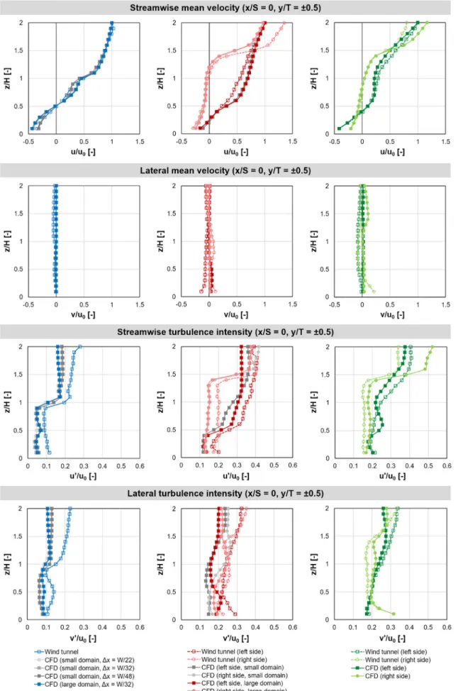
Fig. 8. Comparison of the pointwise velocity and turbulence results between the experiment and the CFD simulations for the three building patterns: uniform canyons (left), matrix towers (middle), and staggered towers (right).
D¼ρσ2
2tdiff ; (10)
in whichtdiff[s] is the temporal length of thefiltering, which was kept constant (10 s) in all cases.
Based on the near-ground or canopy average concentration, the mass Stanton number characterizing the ventilation efficiency of the different building patterns can be obtained as the reciprocal of the mean normalized concentration:
k*¼1
c*: (11)
2.2.4. Solution methods and convergence criteria
For the numerical solution, the Bounded Central Differencing Scheme flux formulation and the SIMPLE (Semi-Implicit Method for Pressure Linked Equations) algorithm were used, along with the Bounded Second Order Implicit scheme for temporal discretization, which are the default options for LES simulations in ANSYS Fluent 19.3 (ANSYS, 2019). The iterative solution was carried on in each time step until the residuals of theflow equations were reduced by at least three orders of magnitude compared to the initial state but in a maximum of 20 iterations. For the unsteady particle tracking in Fluent, the trapezoidal method was utilized for numerical integration. To model the microscale turbulent diffusion, the Discrete Random Walk model was enabled for the particles from all sources, with the time scale constant uniformly set to 0.15 (default value). In the scalar transport equation–used for the spatialfiltering of the concentrationfield–, the second orderflux formulation was used.
3. Results and discussion
3.1. Mesh convergence and the impact of the domain size
The mesh convergence analysis was executed on the model of uni- form canyons using the small domain (see Fig. 6andTable 2for the details). As Large Eddy Simulation is applied, the spatial resolution af- fects–beyond the discretization error–the width of the resolved tur- bulent spectrum, i.e. the boundary between the meso- and microscopic turbulence.
Lower velocities were found within the canyon in the case of the finest mesh (W/Δx¼48), which showed a closer agreement with the measurement data compared to the coarser meshes (W/Δx¼32 and 22).
This can be a consequence of the fact that the relatively thin shear layer at roof height (z/H¼1) is sensitive of the resolution. However, it must be noted that the variation of the numerical results obtained on different meshes falls into the range of the difference between the experimental profiles obtained in different canyons (seeFigs. 8and4, respectively).
The turbulence intensity results did not improve substantially on the finer meshes, which points out that most of the inaccuracies can be attributed to other model parameters.
In terms of the mean concentration distributions, the application of the larger simulation domains (wider and taller domains with the cor- responding propulsion parameters, seeFig. 6andTable 2) substantially improve the agreement with the experimental data, especially in the source canyon of the matrix towers arrangement.
3.2. Validation for velocity and turbulence
The time average and thefluctuation of the streamwise and lateral velocity components were compared (wind tunnel experiments vs. CFD simulations) for all three building patterns in the 0th canyon. For the matrix and staggered tower arrangements, the comparison was carried out behind both a tall and a short building (x¼0;y/T¼ 0.5). The
propulsion side profiles (y/T¼0.5) are indicated with darker, while the ones on the passive side are denoted by lighter colors inFig. 8. The profiles obtained in the smaller domains are shown in greyscale. For each profile, 20 gauging points were used, spaced evenly in the vertical di- rection (z/H¼0.1, 0.2,…, 1.9, 2). Note that the horizontal location of the vertical profiles is identical to that of the sources shown inFig. 3.
It is shown inFig. 8that the normalized mean velocity profiles show good agreement between the experimental and simulation results, characterized by a 95% correlation. The largest differences can be found in the streamwise mean velocity component over roof height in the case of the towers (z/H>1.5), which is a consequence of the horizontally homogeneous driving force being relatively close to the top of the buildings.
The turbulence results of the CFD model display a good qualitative agreement with the wind tunnel data, which can also be seen inFig. 8.
The correlation between the computed and measured turbulence data is 83%. It is shown by both methods that the turbulence intensity is significantly increased below roof height by constructing towers, which suggests that the variable roof height promotes canopy ventilation. There is a remarkable turbulence deficit at the reference location (z/H¼2) which could be mitigated by reducing the time parameter of the model (Ct).
Another source for inaccuracy is that the periodic LES model is only able to generate mesoscopic turbulence caused by the wind shear above the roofs. However, in the wind tunnel, a strong shear layer is formed at the leading edge of the building array (upstream from the 10th canyon), which generates turbulence that can be observed even in the gauging points at the 0th canyon. The existence of such an inner boundary layer was also observed in other wind tunnel experiments, see Castro et al. (2017). The turbulence deficit is less pronounced for the matrix and staggered tower configurations, since more kinetic energy (TKE) is produced by the canopy, suppressing the turbulence originating from the leading edge of the building array.
3.3. Validation for concentration
The lateral concentration distributions are shown inFig. 9, and the vertical profiles are shown inFig. 10. Generally, the model captures the important tendencies of the measured mean concentration distribution.
The correlation coefficient between the measured and computed con- centration data is 0.77.
The best match can be found within the 0th canyons, except for the close vicinity of the sources, which can be explained by the fact that the wind tunnel measurements feature a 28 mm diameter flush-mounted sources, while the particles in the CFD model are injected at a single point. It was found in the framework of the present study that the tem- poral variation of the number of particles in separate street canyons is practically independent of the diameter of the source (tested for 2, 10, and 28 mm).
The mean concentrationfield is generally overestimated within the downstream canyons; furthermore, the concentration boundary layer over the buildings is thinner in the CFD simulations compared to that observed in the wind tunnel measurement, which is the most pronounced in the case of the uniform canyons. The differences might be attributed to the following reasons:
1. In some cases, the turbulent kinetic energy is underestimated, which affects the dispersion as well.
2. Massless particles were used in the simulation, neglecting the positive buoyancy of the methane tracer gas.
3. The bulkflow in the open test section of the wind tunnel entrains air from the canopy. The air escaping the canyons vertically induces a
Fig. 9. Lateral concentration distributions of the three building arrangements: uniform canyons (blue), matrix towers (red), and staggered towers (green). The left and right sources are located aty/T¼ 0.5. Only one source is active at one time. (For interpretation of the references to color in thisfigure legend, the reader is referred to the Web version of this article.)
Fig. 10.Vertical concentration distributions of the three building arrangements: uniform canyons (blue), matrix towers (red), and staggered towers (green). Only one source (left or right) is active at one time. (For interpretation of the references to color in thisfigure legend, the reader is referred to the Web version of this article.)
minor crosswiseflow within the canyons, which is not present in the CFD model (seeFig. 8), causing the additional dilution of the tracer gas.
4. In the low concentration zones, the relative measurement error is higher.
3.4. Comparison of the building patterns 3.4.1. Dispersionfields of different sources
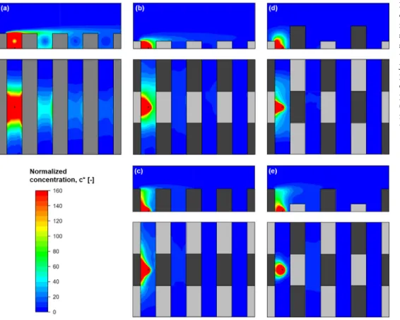
In each street canyon, uniform or not, as a consequence of the canyon vortex (Fig. 11a) or similar rotatingflow structures, the locally emitted pollutants are swept toward the leeward wall, resulting in an imbalance between the pedestrian exposure at the leeward and windward sides.
This asymmetry in concentration is not present in the canyons down- stream from the sources.
The introduction of building height variability generates lateral ve- locity as well as increased turbulence under roof height, therefore pro- moting the dilution of the pollutants. For both tower structures, there is a downwash at the windward side of the tall buildings, which is deflected in both crosswise (y) directions as it reaches ground level. Therefore, diverging streamlines can be observed in front of the tall buildings, thus the pollutants emitted at these locations are spread at street level (Fig. 11cd). On the other hand, as a consequence of the converging streamlines upstream from the short buildings, the pollutants are locally accumulated (Fig. 11be). Regardless of the position of the source; how- ever, in the case of variable roof height, the exposure of the pedestrians and the residents of the nearby buildings are significantly smaller than that of the uniform canyons, and negligible in the subsequent streets according to the model results.
3.4.2. Characteristic vertical profiles
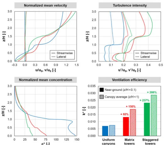
In this section, the periodic building patterns are globally character- ized by the vertical profiles of velocity, turbulence and concentration, obtained by horizontal averaging in one cell thick layers (Δz¼H/32).
InFig. 12 similar near-ground velocity ratios (u/u0, v/u0) can be observed for all periodic building arrangements, but there is significantly more turbulence both in streamwise and in lateral directions when towers are present. The variable roof height results in rougher canopies, which cause smaller velocity gradients atz/H¼1.5 (compared toz/Hfor the uniform canyons), as well as substantially higher turbulence in the boundary layer. Rough building patterns are prone to extract more en- ergy from the atmospheric boundary layer, which leads to a decrease in wind speed in the long run. This effect is not addressed in the present study, in contrast to our previous investigations (Kristof and Füle, 2017).
The Lagrangian approach applied in the present model allows for analyzing the entire dosefield of each source, as the particles are tracked in the infinite space. It is advantageous that the individual vertical con- centration profiles of each investigated raster can be summed to obtain the total footprint of a source, which characterizes the canopy ventilation efficiency. In the present study, for the matrix and staggered towers, two injections are placed in one raster in accordance with the variable roof height; therefore, their combined result was divided by two.
The vertical profiles of mean normalized concentration shown in Fig. 12confirm the superiority of the matrix and the staggered tower arrangements over the uniform street canyons. By constructing buildings of different height while keeping the building volume constant, both the near-ground and canopy average concentrations can be significantly decreased, resulting in substantially more efficient ventilation. The dilution coefficients of the building patterns with variable roof height are
Fig. 11.Mean normalized concentration distributions for the uniform canyons (a), the matrix towers (b – left source, c – right source), and the staggered towers (d–left source, eright source). Wind direction: left to right. The vertical cut planes are located at y/T ¼ 0.5, and the horizontal ones are placed atz/H ¼ 0.05. Darker grey colors denote taller buildings. The positions of the point sources are marked with black dots.
(For interpretation of the references to color in thisfigure legend, the reader is referred to the Web version of this article.)
1.92…3.86 times higher than the corresponding values of the uniform canyons.
3.4.3. Time-dependent particle results
The location of the particles emitted from each source was recorded in every 0.05 s, which served as a basis for calculating the time-dependent particle counts in thefirst few canyons. The investigated volumes for all three building patterns can be defined byx/S2[i–0.25,iþ0.25] andz/
H2[0, 1]–identical to the below-roof part of the uniform canyons–with ibeing the number of the canyon of interest.
As discussed in Section2.2.3, there are two types of sources placed in the domains: continuous point-like emissions, injecting one particle per time step; and spatially distributed sources of 28 mm diameter, injecting 1000 particles simultaneously, at six different times (2, 3, and 4 s offlow time, at the beginning and the end of the time step).Fig. 13shows the particle count relative to the total number of particles emitted from either the steady or the pulse-like sources during the entire simulation (Nall,steady and Nall,pulse, respectively). Each of the curves ofFig. 13b shows the average of the six particle clouds, with theflow time relative to the time of emission (t0).
It can be seen in Fig. 13a, that the average number of particles accumulating in the source canyons are substantially lower for the matrix (left source:43%, right source:55%) and the staggered towers (left:
62%, right:80%) compared to the uniform canyons. Similar ten- dencies can be observed in the downstream canyons; however, it must be noted that the mean particle count in the subsequent streets is one order of magnitude smaller. In this regard, it does not seem crucial that the extreme values corresponding to the staggered, and especially, the matrix towers can exceed the extremities of the uniform canyons. The curves also reveal that far from the source canyon, the particle clouds emitted from the left and right sources show increasing correlation; i.e., the point
of origin has a decreasing influence–as expected based on the obser- vations ofXie and Castro (2009).
Fig. 13b shows how particles emitted from pulse-like sources (such as pollutants from a bus stop, or aerosols from a sneeze) escape the canopy.
It can be concluded that it takes less time for the particles in the matrix and especially in the staggered arrangement to clear the 0th canyon compared to the uniform canyons. Similar tendencies can be observed in the downstream streets, and the rates of the pollutants escaping the 0th canyon after switching off the continuous sources also show an analogous behavior inFig. 13a. The particle reflux into the subsequent canyons is lower for the uniform canyons relative to the towers, resulting in lower maxima of the corresponding curves inFig. 13b. But, again, the pedes- trian exposure in the downstream streets is at least one order of magni- tude lower, thus this effect is less important.
The particle count in a control volume can be interpreted as con- centration, and the integral of the curves give the corresponding dose values. The area below the corresponding curves betweenFigs. 13a andb is practically identical for the entire length of the simulation, supporting the approach that the dispersionfield of spatially and temporally inho- mogeneous emissions can be constructed via the convolution of the concentration responses of the individual sources.
4. Conclusions and outlook
The technical objective of the present study is the assessment of the ventilation efficiency of three periodic building patterns of equal total volume: uniformH/W¼1 street canyons and a combination of 0.5Hand 1.5Hhigh towers, both in matrix, and in staggered arrangement. The investigation was carried out via wind tunnel experiments and numerical modeling, namely, the Transient Wind Forcing model introduced by the previous work of the authors (Kristof et al., 2020).
Fig. 12. Characteristic vertical profiles and ventilation efficiencies of the investigated periodic building patterns. The vertical profiles are obtained by averaging the field variables inH/32 thick horizontal layers.
The TWF model utilizes periodic boundary conditions to simulate the flowfield around the periodically repeated buildings. It is an important feature of the model that due to the time-dependent measurement-based propulsion of theflow, the macroscale turbulence–in other words, the flow structures exceeding the domain size–can also be taken into ac- count. It was shown that at the center of the propulsion around 70% of the TKE is contained in these large-scale eddies. The TWF model utilizes Lagrangian particle tracking to simulate the dispersion of air pollutants emitted from near-ground sources. The number of periodic jumps in thex and in theydirection is recorded for each particle; therefore, their path can be followed outside the borders of the original periodic domain.
Based on the local residence time of the particles, the pollutant dose distribution for both steady and pulse-like emissions can be calculated in the horizontally unlimited space. The present investigation is also aimed at the validation of the TWF-based aperiodic dispersion model.
Note that the accuracy of TWF model results is also affected by the correct choice of the model parameters (Ct,CL,z0,X,Y,Z). The present research did not cover the full optimization of these model parameters due to the high computational demand of LES calculations.
During the validation, it was shown that the velocity and turbulence intensity profiles characterizing theflowfield are reproduced with good accuracy (correlation coefficients: 95% and 83%, respectively). Based on the periodicflowfields, the aperiodic dose distribution–caused by point- like sources–was calculated. The mean normalized concentration dis- tribution also showed good correspondence with the measurement data, especially in the source canyons, which are the most critical locations in terms of pedestrian exposure to traffic-induced air pollutants. Reasonable agreement was found between the experimental and simulation results, characterized by a 77% correlation.
Furthermore, the time-dependent particle counts within the street canyons was analyzed, which indicated the superiority of the matrix and
staggered towers compared to the uniform canyons, both for steady and for pulse-like sources. It was observed for both the matrix and staggered tower structures that the particles are able to escape the source canyon significantly faster compared to the uniform canyons; therefore, the time- average of the normalized particle count below average roof height is reasonably lower in the source canyon (matrix towers: 50%; staggered towers: 70%). Since the cumulative dispersion field of spatially and temporally inhomogeneous emissions can be constructed via the convolution of the concentration responses of point sources, similar to the ones presented in this paper, they can be crucial input data for operational forecast systems.
It was shown by normalized concentration results of the CFD model that the variation of the roof height can significantly improve the ventilation of the periodic building configurations. It was concluded, the near-ground and the canopy average concentrations show a 48…70%
decrease for the matrix tower arrangement, and a 60…74% decrease for the staggered tower arrangement compared to the uniform canyons, while the total building volume is kept constant between the three cases.
The presented dispersion model is capable of taking the dynamic changes in wind direction and magnitude into account; therefore, the accuracy of the TWF model can potentially exceed the limitations of wind tunnel tests.
CRediT authorship contribution statement
Balint Papp:Conceptualization, Methodology, Software, Validation, Formal analysis, Resources, Writing - original draft, Writing - review&
editing, Visualization, Supervision, Project administration, Funding acquisition.Gergely Kristof:Conceptualization, Methodology, Software, Writing - original draft, Writing - review&editing, Supervision, Project administration, Funding acquisition. Balazs Istok: Methodology, Fig. 13. Particle count in different canyons (0th, 1st, 4th) for different building patterns, normalized by the total number of particles emitted from the sources. Left:
continuous emission of 1 particle per time step. Right: pulse-like emissions of 61000 particles for each curve.