Brain Tumor Segmentation from Multi-Spectral Magnetic Resonance Image Data Using an Ensemble Learning Approach
Agnes Gy˝orfi, Szabolcs Csaholczi, T´ımea F¨ul¨op, Levente Kov´acs and L´aszl´o Szil´agyi´
Abstract— The automatic segmentation of medical images represents a research domain of high interest. This paper proposes an automatic procedure for the detection and segmen- tation of gliomas from multi-spectral MRI data. The procedure is based on a machine learning approach: it uses ensembles of binary decision trees trained to distinguish pixels belonging to gliomas to those that represent normal tissues. The classification employs 100 computed features beside the four observed ones, including morphological, gradients and Gabor wavelet features.
The output of the decision ensemble is fed to morphological and structural post-processing, which regularize the shape of the detected tumors and improve the segmentation quality. The proposed procedure was evaluated using the BraTS 2015 train data, both the high-grade (HG) and the low-grade (LG) glioma records. The highest overall Dice scores achieved were 86.5%
for HG and 84.6% for LG glioma volumes.
Index Terms— magnetic resonance imaging, brain tumor, tumor detection, image segmentation, ensemble learning.
I. INTRODUCTION
Brain tumor represents a major cause of death in both de- veloped and developing countries [1]. There are two general categories of brain tumors: the so-called high-grade (HG) and low-grade (LG) gliomas. Patients diagnosed with HG glioma live fifteen more months in average. On the other hand, it is possible to live several years with a low-grade glioma. A key factor of survival or better life expectancy represents the early diagnosis. This is why there is a strong need for algorithms that can reliably detect the presence of
*This project was supported in part by the Sapientia Institute for Research Programs. This project has received funding from the European Research Council (ERC) under the European Unions Horizon 2020 research and innovation programme (grant agreement No 679681), and Project no. 2019- 1.3.1-KK-2019-00007, implemented with the support provided from the National Research, Development and Innovation Fund of Hungary, financed under the 2019-1.3.1-KK funding scheme. The work of T. F¨ul¨op was supported by the Collegium Talentum 2019 Programme of Hungary. The work of L. Szil´agyi was supported by the Hungarian Academy of Sciences through the J´anos Bolyai Fellowship program.
A.´ Gy˝orfi is with Doctoral School of Applied Informatics (AIAMDI), Obuda´ University, B´ecsi ´ut 96/b, H-1034 Budapest, Hungary (phone/fax: +36-1-666-5585; e-mail: gyorfi.agnes at phd.uni-obuda.hu).
L. Kov´acs and L. Szil´agyi are with University Research, Innovation, and Service Center (EKIK), ´Obuda University, B´ecsi ´ut 96/b, H-1034 Budapest, Hungary (phone/fax: +36-1-666-5585; e-mail: {kovacs.levente, szilagyi.laszlo} at nik.uni-obuda.hu).
A. Gy˝orfi and L. Szil´agyi are also with Dept. of Electrical En-´ gineering, Sapientia University, Calea Sighis¸oarei 1/C, 540485 Tˆırgu Mures¸, Romania (phone: +40-265-206-210; fax: +40-265-206-211; e-mail:
{gyorfiagnes,lalo} at ms.sapientia.ro).
Sz. Csaholczi and T. F¨ul¨op are with Dept. of Mathematics- Informatics, Sapientia University, Calea Sighis¸oarei 1/C, 540485 Tˆırgu Mures¸, Romania (phone: +40-265-206-210; fax: +40-265-206-211; e- mail: {szabolcscsaholczi55,fuloptimea1427} at gmail.com).
tumors in MRI data, even when it is in an early phase.
The quickly growing number of MRI devices deployed in hospitals and the even quicker rising amount of collected MRI data brought another attribute to the specification: the newly developed algorithms need to be fully automatic, so that they can separate surely negative cases from suspected positive ones, and thus can help the medical expert focus on the serious cases.
Recently developed algorithms for glioma detection and segmentation mostly rely on multi-spectral magnetic reso- nance imaging (MRI), which might be a direct consequence of the BraTS Challenges organized jointly with the MICCAI conference since year 2012 [2], [3]. A comprehensive sum- mary of earlier brain tumor segmentation solutions based on MRI data can be found in the review paper published by Gordillo et al. in [4]. Recently published solutions usually combine advanced unsupervised image segmentation algorithms with supervised and semi-supervised machine learning techniques. The wide spectrum of methodologies includes: active contour models combined with texture fea- tures [5], cellular automata combined with level sets [6], graph cut segmentation algorithm [7], superpixels combined with non-parametric classifiers [8], feature fusion combined with joint label fusion [9], texture feature and kernel sparse coding [10], Gaussian mixture models [11], [12], fuzzy c- means clustering in semi-supervised context [13], [14], fuzzy c-means clustering combined with region growing [15], AdaBoost classifier [16], extremely random trees (ERT) [17]
combined with superpixel level features [18], random forests [19], [20], [21] and ensemble of random forests [22], support vector machines [23], expert systems [24], convolutional neural network [25], [26], deep neural networks [27], [28], [29], [30], generative adversarial networks [31], and tumor growth model [32].
This paper proposes a brain tumor segmentation procedure that employs an ensemble learning approach based on binary decision trees, and a twofold post-processing that uses mor- phological and structural criteria to regularize the shape of the detected tumor and to enhance the segmentation quality.
Compared to our previous works [33], the main novelty consists in the structural post-processing, which individually evaluates each contiguous tumor region within the brain volume based on its size and shape. The procedure is trained and evaluated using the MICCAI BraTS 2015 train data set, both the LG and HG glioma records.
The rest of the paper is structured as follows: section II presents the details of the proposed segmentation procedure, dedicating a subsection to each processing step. Section III
evaluates the segmentation accuracy of the proposed pro- cedure based on experiments conducted using two publicly available MRI data sets. Section IV concludes the study.
II. MATERIALS AND METHODS
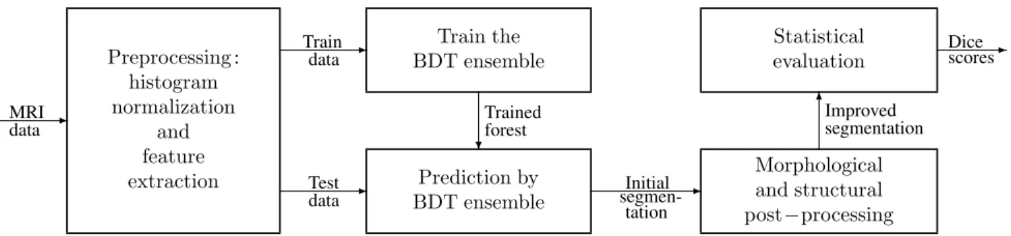
The steps of proposed method are exhibited in Figure 1.
All MRI data volumes involved in this study go through a multi-step preprocessing, whose main goal is to provide uniform histograms to all volumes, and to generate further features to all pixels. After separating train data records from test data records, the former is fed to the ensemble learning step. Trained ensembles of binary decision trees are used to provide prediction for the pixels of the test data records. A twofold post-processing is employed to regularize the shape of the estimated tumor. Finally, statistical markers are used to evaluate the accuracy of the whole proposed procedure.
A. Data
The multi-spectral MRI volumes of the BraTS 2015 data set [2], [3] include NLG = 54 low-grade and NHG = 220 high-grade glioma records. Each record consists of four observed data channels (T1, T2, T1C, FLAIR) and the ground truth established by human experts using a semi- automatic procedure presented in [2]. In case of each record, all data channels were registered to the T1 using a standard automatic procedure. Volumes consist of 155 slices, each slice containing 240×240 pixels. Pixels are isovolumetric, each of them represents a one millimeter sized cubic area of brain tissues. Since the adult human brain has a volume of approximately1500cm3, the number of pixels is each record ranges around 1.5 millions. Each record contains gliomas, the volume of lesions ranges between10and300cm3. Some of the records intentionally contain missing or altered values, in the amount of up to one third of the pixels in one of the four data channels.
B. Pre-processing
Pre-processing theoretically has the main goal to deal with two possible type of noise:
• The intensity non-uniformity (INU) of the MR image data is mainly the manifestation of turbulence of the magnetic field [34], [35], [36]. Our procedure uses the method of Tustisonet al.[37] to suppress the effects of INU.
• The great variety of the intensity ranges is another ob- stacle encountered in MRI data. The absolute intensity value of a pixel has no meaning by itself. We treat the MRI volumes and their data channels independently of each other, using a context dependent linear transform.
The linear coefficients are chosen such a way that the 25-percentile and 75-percentile value is mapped to 600 and 800, respectively. Further on, transformed intensity values are bounded at 200 on the lower end, and at 1200 on the upper end of the target interval. Details are presented in our previous work [33].
The four observed features of each pixel do not contain enough information for an accurate classification. Neighbour
pixels in the slices of any volume highly correlate with each other. Further on, the registration of the four data channels in each record can hardly be called perfect. These are some reasons that motivate the generation of several morphological features from the planar and spatial neighborhood of each pixel. Our procedure generates 25 computed features each pixel in each data channels. Thus the total number of features that characterize each pixel is 104. The generated features for every pixel in every data channel are:
• average, minimum and maximum values extracted from 3×3×3 spatial neighborhood;
• five average and five median values extracted from planar neighborhoods of sizes ranging from 3×3 to 11×11;
• four gradient features extracted from 7 × 7 planar neighborhood, with respect to the four main directions;
• eight Gabor wavelet features extracted from 11×11 planar neighborhood.
C. Decision making
The total number ofNρrecords (54 or 220, for LG and HG data sets, respectively) is randomly separated into two equal groups. These groups serve as train and test data in turns for the decision making algorithm. The train data is fed to the ensemble learning process. The ensemble we employed in this study is built from binary decision trees [38], which share the following main characteristics:
• The number of the trees in the ensemble is previously set tonT = 125. This value was determined empirically during previous investigations [33].
• The number of feature vectors used to train each tree, denoted by nF, was chosen from the set {100k,200k,500k,1000k}. Simulations were per- formed with all these values to establish which has the best outcome in terms of accuracy and efficiency.
• The set of nF randomly selected feature vectors in- volved into the training of each BDT contained p− percent of negatives and p+ = 100 −p− percent of positives. The adequate parameter values of the mixture were established empirically during previous investigations [33].
• BDTs are built using an entropy-based criterion, allow- ing the tree to grow as deep as necessary to provide perfect separation of positive and negative feature vec- tors. The maximum depth of trees range between 25 and 45, depending on the train data size (nF) and the random train data.
When the ensemble is trained, the test data records are fed to the ensemble for prediction. The feature vector of each pixel from the test data set receives a vote from each BDT of the ensemble, collecting a total number ofnT votes.
The ensemble decision for the test pixel is established by the majority of the individual votes received from the trees. The ensemble thus gives a label to each test pixels. These labels are considered intermediary, because they may be overruled during the post-processing.
Statistical evaluation
Morphological and structural post−processing Prediction by
BDT ensemble Preprocessing :
histogram normalization
and feature extraction
Train the BDT ensemble
-
-
- -
6
? MRI
data
Train data
Test data
Initial segmen-
tation
Improved segmentation
Dice- scores
Trained forest
Fig. 1. Schematic representation of the proposed method.
D. Post-processing
The proposed post-processing step has the goal of giving the detected lesions a regularized shape, which is likely to improve the accuracy of the segmentation. The post- processing is performed in two phases:
1) The morphological phase reevaluates the intermediary label of each pixel from the test data set. A cubic neighborhood of size11×11×11is defined with the current pixel in central position. The number of valid brain pixels within the neighborhood in denoted bynτ, while the number of pixels with positive intermediary label within the neighborhood by nπ. The new label of the current pixel is set to positive ifnπ/nτ>1/3.
The threshold value was established empirically.
2) The structural phase of the post-processing has the option to discard some of the positive labels but never produces extra positive labels. After the mor- phological phase, adjacent pixels with positive labels compose some contiguous formations (regions) within the volume. As a first operation we identify all such the contiguous lesions using a spatial region growing method. Those lesions which contain less than 100 pixels are discarded by default, because they are too small to be reliable declared gliomas. In case of larger lesions, principal component analysis (PCA) is applied to the coordinates of all pixels that form the lesion, to establish the three main spacial axis and the sizes in each of these directions. PCA provides three eigenvalues λ1 > λ2 > λ3, where the radius of the contiguous lesion in the three directions are√
λ1,√ λ2
and√
λ3. If the smallest radius of the region is smaller than a predefined threshold (√
λ3 < 2), the current detected lesion is discarded. All detected lesions that survive the discarding criteria enumerated above, are finally declared positives, and all pixels belonging to them are finally labelled accordingly.
E. Evaluation criteria
The total number of MRI records involved in a certain study scenario is Nρ ∈ {NLG, NHG}. Since the train and test data sets can swap their roles, we can perform test segmentation for all Nρ records. Let Γ(π)i andΓ(ν)i denote the set of positive and negative pixels within volume i (i= 1. . . Nρ), according to the ground truth. Moreover, let
TABLE I
STATISTICAL CRITERIA TO EVALUATE SEGMENTATION QUALITY OF INDIVIDUAL VOLUMES
Indicator Formula
Dice score DSi=2×|Γ
(π) i ∩Λ(π)
i |
|Γ(π) i |+|Λ(π)
i |
Sensitivity TPRi=|Γ
(π) i ∩Λ(π)
i |
|Γ(π) i |
Specificity TNRi=|Γ
(ν) i ∩Λ(ν)
i |
|Γ(ν) i |
Accuracy ACCi=|Γ
(π) i ∩Λ(π)
i |+|Γ(ν) i ∩Λ(ν)
i |
|Γ(π) i |+|Γ(ν)
i |
Λ(π)i and Λ(ν)i stand for the set of pixels of volume i that received positive and negative final labels, respectively. The cardinality of any finite setZ is denoted by|Z|.
The main accuracy markers that we extract from volumei, are defined as presented in Table I. These statistical markers range from 0 to 1. Ideal segmentation is represented by the maximum value of each marker.
To characterize the accuracy of segmentation for a whole set of records, we may compute the average value of the four markers, with the general formula
X = 1 Nρ
Nρ
X
i=1
Xi , (1)
whereX ∈ {TPR,TNR,DS,ACC}.
The overall Dice Score, denoted by DS, is given by thef formula:
DS =f 2×
Nρ
S
i=1
Γ(π)i ∩
Nρ
S
i=1
Λ(π)i
Nρ
S
i=1
Γ(π)i
+
Nρ
S
i=1
Λ(π)i
. (2)
III. RESULTS AND DISCUSSION
The proposed brain tumor segmentation procedure under- went a thorough experimental evaluation involving the set of 54 LG tumor records and the set of 220 HG tumor records of the BraTS 2015 data set separately. Tests were performed using four different values of the train data sizenF that was used for the training of each BDT: 100k, 200k, 500k, and
TABLE II
MAIN GLOBAL AND INDIVIDUAL ACCURACY INDICATORS
Low-grade glioma volumes High-grade glioma volumes
Accuracy Train data size per BDT (nF) Train data size per BDT (nF)
indicator 100k 200k 500k 1000k 100k 200k 500k 1000k
Overall Dice score DSf 85.77% 86.12% 86.26% 86.50% 83.91% 84.27% 84.44% 84.60%
Average Dice score DS 83.78% 83.97% 84.06% 84.27% 79.46% 80.28% 80.66% 80.90%
Average sensitivity TPR 79.82% 80.36% 80.83% 81.36% 76.25% 77.73% 78.24% 78.63%
Average specificity TNR 99.41% 99.38% 99.35% 99.32% 99.16% 99.08% 99.07% 99.05%
Correct decision rate ACC 98.11% 98.15% 98.16% 98.18% 97.79% 97.82% 97.84% 97.85%
DSi>90% 16 of 54 16 of 54 18 of 54 18 of 54 72 of 220 70 of 220 70 of 220 71 of 220 DSi>85% 38 of 54 39 of 54 40 of 54 40 of 54 120 of 220 122 of 220 124 of 220 124 of 220 DSi>80% 44 of 54 44 of 54 44 of 54 45 of 54 149 of 220 153 of 220 154 of 220 154 of 220 DSi>70% 49 of 54 48 of 54 48 of 54 49 of 54 179 of 220 180 of 220 180 of 220 181 of 220 DSi>60% 50 of 54 50 of 54 50 of 54 50 of 54 194 of 220 197 of 220 198 of 220 199 of 220 DSi>50% 51 of 54 51 of 54 51 of 54 52 of 54 203 of 220 206 of 220 207 of 220 207 of 220
Tumor size (cm3)
0 30 60 90 120 150 180 210 240 270
Dice score (%)
30 40 50 60 70 80 90
100 LG tumor volumes
Fig. 2. Dice scores obtained for individual low-grade tumor values, plotted against the true size of the tumor.
Tumor size (cm3)
0 30 60 90 120 150 180 210 240 270 300 330
Dice score (%)
0 10 20 30 40 50 60 70 80 90
100 HG tumor volumes
Fig. 3. Dice scores obtained for individual high-grade tumor values, plotted against the true size of the tumor.
1000k. The rate of negatives in the train data was set to p−= 93%in case of the LG data, andp−= 91%in case of the HG records. The segmentation accuracy was evaluated for each individual record using the statistical indicators presented in Section II-E, and global indicator values were extracted to be able to formulate assertions on the overall performance. Detailed results are presented in the following.
Table II presents statistical characteristics of the global performance of the proposed segmentation procedure. The upper part of the table exhibits the overall and average Dice score, and the average sensitivity, specificity and correct decision rate obtained in case of various train data sizes. Dice score and sensitivity values grow together with the train data
Individual LG volumes in increasing order of the accuracy indicators
0 9 18 27 36 45 54
Dice score and sensitivity (%)
20 30 40 50 60 70 80 90 100
Accuracy indicators obtained for individual LG volumes
Dice score Sensitivity
0 9 18 27 36 45 54
Specificity and accuracy (%)
86 88 90 92 94 96 98 100
Specificity Accuracy
Fig. 4. Statistical accuracy indicator values obtained for the 54 low-grade tumor volumes separately, represented in increasing order.
Individual HG volumes in increasing order of the accuracy indicators
0 55 110 165 220
Dice score and sensitivity (%)
0 10 20 30 40 50 60 70 80 90 100
Dice score Sensitivity
0 55 110 165 220
Specificity and accuracy (%)
90 91 92 93 94 95 96 97 98 99 100
Accuracy indicators obtained for individual HG volumes
Specificity Accuracy
Fig. 5. Statistical accuracy indicator values obtained for the 220 high-grade tumor volumes separately, represented in increasing order.
size, while the specificity and correct decision rate had only slight variations.
The lower part of Table II indicates, in case of how many individual MRI records the proposed method produced a segmentation having a Dice score exceeding various prede- fined threshold values ranging between 50% and 90%. These numbers also indicate that larger train data sets produce en- sembles that give better accuracy at prediction. The proposed segmentation procedure achieves Dice scores above 80% in case of 80% of LG glioma volumes and 70% of HG glioma volumes.
Figure 2 shows the Dice scores obtained for individual LG glioma volumes, plotted against the true size of the
Fig. 6. One slice from ten different HG tumor volumes, the four observed data channels and the segmentation result. The first four rows present the T1, T2, T1C and FLAIR channel data of the chosen slices. The bottom row exhibits the segmented slice, representing true positives (|Γ(π)i ∩Λ(π)i |) in green, false negatives (|Γ(π)i ∩Λ(ν)i |) in red, false positives (|Γ(ν)i ∩Λ(π)i |) in blue, and true negatives (|Γ(ν)i ∩Λ(ν)i |) in gray, whereiis the index of the current MRI record.
tumor, as indicated by the human expert made ground truth.
Each cross (×) represents a Dice score, while the dashed line shows the linear trend identified via linear regression.
The trend indicates that Dice scores are slightly higher for larger tumors, but even for the small ones, the expected value is well above 80%. There are some LG tumor records for which the high accuracy was not achieved. Those with lots of missing data belong to this category.
A similar representation of Dice scores achieved for indi- vidual HG glioma volumes is given in Fig. 3. The distribution of Dice score values is quite similar to the Dice scores of LG data. However, the linear trend rises steeper with tumor size, and small gliomas have somewhat lower expected Dice scores, around 75%. Here there are also two records with Dice scores below 10%, which contain image data of very low quality. Nevertheless, the vast majority of records received a fine segmentation, with Dice scores above 80%.
Figure 4 plots the main accuracy indicator values obtained for individual LG tumor records in increasing order: Dice score and sensitivity on the left side, specificity and accuracy (correct decision rate) on the right side, to provide good visibility. Figure 5 plots the same graphs with the accuracy indicators achieved in case of the HG tumor volumes. These graphs reveal several important facts:
• The distribution of Dice scores shows that the median value is well above the average: the difference is around 2%for the LG data and4%for the HG data. The median Dice score is well approximated by the overall value DS.f
• Specificity values are above 99% in average, and the values obtained for individual records are above 99%
in a vast majority of cases. This is important because of the high number of negative pixels. Without this feature the proposed procedure would produce lots of false positives.
• Correct decision rates are around98% in average. This
TABLE III
COMPARISON WITH STATE-OF-THE-ART METHODS Method (Classifier) Year BraTS data Dice scores Tustisonet al.[19] (RF) 2015 2013 DS= 0.87 Pereiraet al.[25] (CNN) 2016 2013 DS= 0.88 Pintoet al.[17] (ERT) 2018 2013 DS= 0.85 Pereiraet al.[25] (CNN) 2016 2015 DS= 0.78 Zhaoet al.[29] (CNN) 2018 2015 DS= 0.84 Peiet al.[9] (RF, boosting) 2020 2015 DS= 0.850
2015 LG DS= 0.843
Proposed method DSf = 0.865
(BDT ensemble)
2015 HG DS= 0.809 DSf = 0.846
means that only one out of fifty pixels is misclassified.
Figures 2 - 5 all represent the accuracy indicator values obtained in case of training the BDTs with one million feature vectors.
Figure 6 shows the final outcome of the segmentation on ten selected slices from different MRI records. Each column relates on a single slice. The upper four rows show the augmented input data of the four data channels, while the bottom row indicates the segmentation results, using color coding described in the figure caption.
To perform the test on a new record that was never seen by the trained procedure needs between 100 and 120 seconds, depending on the train data size and the number of pixels in the test record. This duration is achieved on a current notebook computer with i7 processor, running at 2.6 GHz frequency. The software is executed on a single core, and no relevant effort was made to optimize the efficiency of the procedure. Approximately half of this time is taken by the feature generation process, which could be easily reduced by replacing the median features with others that can be extracted more efficiently.
IV. CONCLUSIONS
This paper proposed an automatic procedure based on ensemble learning, aimed at the detection and segmentation of brain tumors from multi-spectral MRI records. The seg- mentation was achieved in three phases. The first prepro- cessing step accomplished the data enhancement and feature generation tasks. In the second phase, an ensemble of binary decision trees was trained to separate pixels belonging to lesions from normal tissues, thus providing an intermediary label for each pixel. Finally, a twofold post-processing was applied to refine the intermediary labels and provide regular- ized shape to the detected gliomas. The proposed procedure was built and evaluated using the BraTS 2015 train data, which consists of a total number of 274 glioma records. The highest overall Dice scores, 86.5% for HG and 84.6% for LG glioma volumes, were achieved using the ensemble built with the largest employed train data set. These Dice scores represent 1-1.5% improvement compared to our previous works, and seem competitive with respect to state-of-the-art methods, as indicated in Table III.
REFERENCES
[1] G. Mohan and M. Monica Subashini, “MRI based medical image analysis: Survey on brain tumor grade classification,” Biomed. Sign.
Proc. Contr., vol. 39, pp. 139–161, 2018.
[2] B. H. Menze, A. Jakab, S. Bauer, J. Kalpathy-Cramer, K. Farahani, J. Kirby et al., “The multimodal brain tumor image segmentation benchmark (BRATS),”IEEE Trans. Med. Imag., vol. 34, pp. 1993–
2024, 2015.
[3] S. Bakas, M. Reyes, A. Jakab, S. Bauer, M. Rempfler, A. Crimi et al., “Identifying the best machine learning algorithms for brain tumor segmentation, progression assessment, and overall survival prediction in the BRATS challenge,” arXiv: 1181.02629v2, 19 Mar 2019.
[4] N. Gordillo, E. Montseny and P. Sobrevilla, “State of the art survey on MRI brain tumor segmentation,”Magn. Reson. Imaging, vol. 31, pp. 1426–1438, 2013.
[5] J. Sahdeva, V. Kumar, I. Gupta, N. Khandelwal and C. K. Ahuja, “A novel content-based active countour model for brain tumor segmenta- tion,”Magn. Reson. Imaging, vol. 30, pp. 694–715, 2012.
[6] A. Hamamci, N. Kucuk, K. Karamam, K. Engin and G. Unal, “Tumor- Cut: segmentation of brain tumors on contranst enhanced MR images for radiosurgery applications,”IEEE Trans. Med. Imag., vol. 31, pp.
790–804, 2012.
[7] I. Njeh, L. Sallemi, I. Ben Ayed, K. Chtourou, S. Lehericy, D.
Galanaud and A. Ben Hamida, “3D multimodal MRI brain glioma tumor and edema segmentation: a graph cut distribution matching approach,”Comput. Med. Imag. Graph., vol. 40, pp. 108–119, 2015.
[8] Z. U. Rehman, S. S. Naqvi, T. M. Khan, M. A. Khan and T. Bashir,
“Fully automated multi-parametric brain tumour segmentation using superpixel based classification,”Expert Syst. Appl, vol. 118, pp. 598–
613, 2019.
[9] L. M. Pei, S. Bakas, A. Vossough, S. M. S. Reza, C. Murala and K. M.
Iftekharuddin, “Longitudinal brain tumor segmentation prediction in MRI using feature and label fusion,”Biomed. Sign. Proc. Contr., vol.
55, 101648, 2020.
[10] J. J. Tong, Y. J. Zhao, P. Zhang, L. Y. Chen and L. R. Jiang, “MRI brain tumor segmentation based on texture features and kernel sparse coding,”Biomed. Sign. Proc. Contr., vol. 47, pp. 387–392, 2019.
[11] J. Juan-Albarrac´ın, E. Fuster-Garcia, J. V. Manj´on, M. Robles, F.
Aparici, L. Mart´ı-Bonmat´ı and J. M. Garc´ıa-G´omez, “Automated glioblastoma segmentation based on a multiparametric structured unsupervised classification,”PLoS ONE, vol. 10(5), e0125143, 2015.
[12] B. H. Menze, K. van Leemput, D. Lashkari, T. Riklin-Raviv, E.
Geremia, E. Alberts, et al., “A generative probabilistic model and dis- criminative extensions for brain lesion segmentation – with application to tumor and stroke,”IEEE Trans. Med. Imag., vol. 35, pp. 933–946, 2016.
[13] L. Szil´agyi, S. M. Szil´agyi, B. Beny´o and Z. Beny´o, “Intensity inhomogeneity compensation and segmentation of MR brain images using hybridc-means clustering models”,Biomed. Sign. Proc. Contr., vol. 6, no. 1, pp. 3–12, 2011.
[14] L. Szil´agyi, L. Lefkovits and B. Beny´o, “Automatic brain tumor segmentation in multispectral MRI volumes using a fuzzy c-means cascade algorithm”, Proc. 12th International Conference on Fuzzy Systems and Knowledge Discovery(FSKD 2015, Zhangjiajie, China), pp. 285-291, 2015.
[15] Q. N. Li, Z. F. Gao, Q. Y. Wang, J. Xia, H. Y. Zhang, H. L. Zhang, H. F. Liu and S. Li, “Glioma segmentation with a unified algorithm in multimodal MRI images,”IEEE Access, vol. 6, pp. 9543–9553, 2018.
[16] A. Islam, S. M. S. Reza and K. M. Iftekharuddin, “Multifractal texture estimation for detection and segmentation of brain tumors,” IEEE Trans. Biomed. Eng., vol. 60, pp. 3204–3215, 2013.
[17] A. Pinto, S. Pereira, D. Rasteiro and C. A. Silva, “Hierarchical brain tumour segmentation using extremely randomized trees,”Patt.
Recogn., vol. 82, pp. 105–117, 2018.
[18] T. Imtiaz, S. Rifat, S. A. Fattah and K. A. Wahid, “Automated brain tumor segmentation based on multi-planar superpixel level features extracted from 3D MR images,” IEEE Access, vol. 8, pp. 25335–
25349, 2020.
[19] N. J. Tustison, K. L. Shrinidhi, M. Wintermark, C. R. Durst, B. M.
Kandel, J. C. Gee, M. C. Grossman and B. B. Avants, “Optimal symmetric multimodal templates and concatenated random forests for supervised brain tumor segmentation (simplified) with ANTsR,”
Neuroinformics, vol. 13, pp. 209–225, 2015.
[20] L. Lefkovits, Sz. Lefkovits, L. Szil´agyi, “Brain tumor segmentation with optimized random forest,”Proc. 2nd International Workshop on Brainlesion: Glioma, Multiple Sclerosis, Stroke and Traumatic Brain Injuries(BraTS MICCAI 2016, Athens),Lecture Notes in Computer Science, vol. 10154, pp. 88–99, 2017.
[21] Sz. Lefkovits, L. Szil´agyi, L. Lefkovits, “Brain tumor segmentation and survival prediction using a cascade of random forests,”Proc. 4th International Workshop on Brainlesion: Glioma, Multiple Sclerosis, Stroke and Traumatic Brain Injuries(BraTS MICCAI 2018, Granada), Lecture Notes in Computer Science, vol. 11384, pp. 334–345, 2019.
[22] A. Phophalia and P. Maji,“Multimodal brain tumor segmentation using ensemble of forest metod,” Proc. 3rd International Workshop on Brainlesion: Glioma, Multiple Sclerosis, Stroke and Traumatic Brain Injuries (BraTS MICCAI 2017, Quebec City), Lecture Notes in Computer Science, vol. 10670, pp. 159–168, 2018.
[23] N. Zhang, S. Ruan, S. Lebonvallet, Q. Liao and Y. Zhou, “Kernel feature selection to fuse multi-spectral MRI images for brain tumor segmentation,”Comput. Vis. Image Understand., vol. 115, pp. 256–
269, 2011.
[24] E. Sert and D. Avci, “Brain tumor segmentation using neutrosophic expert maximum fuzzy-sure entropy and other approaches,”Biomed.
Sign. Proc. Contr., vol. 47, pp. 276–287, 2019.
[25] S. Pereira, A. Pinto, V. Alves and C. A. Silva, “Brain tumor segmenta- tion using convolutional neural networks in MRI images,”IEEE Trans.
Med. Imag., vol. 35, pp. 1240–1251, 2016.
[26] H. C. Shin, H. R. Roth, M. C. Gao, L. Lu, Z. Y. Xu, I. Nogues, J. H.
Yao, D. Mollura and R. M. Summers, “Deep convolutional neural networks for computer-aided detection: CNN architectures, dataset characteristics and transfer learning,”IEEE Trans. Med. Imag., vol.
35, pp. 1285–1298, 2016.
[27] G. Kim, “Brain tumor segmentation using deep fully convolutional neural networks,”Proc. 3rd International Workshop on Brainlesion:
Glioma, Multiple Sclerosis, Stroke and Traumatic Brain Injuries (BraTS MICCAI 2017, Quebec City),Lecture Notes in Computer Science, vol. 10670, pp. 344–357, 2018.
[28] Y. X. Li and L. L. Shen, “Deep learning based multimodal brain tumor diagnosis,”Proc. 3rd International Workshop on Brainlesion: Glioma, Multiple Sclerosis, Stroke and Traumatic Brain Injuries(BraTS MIC- CAI 2017, Quebec City), Lecture Notes in Computer Science, vol.
10670, pp. 149–158, 2018.
[29] X. M. Zhao, Y. H. Wu, G. D. Song, Z. Y. Li, Y. Z. Zhang, and Y.
Fan, “A deep learning model integrating FCNNs and CRFs for brain tumor segmentation”,Med. Image Anal., vol. 43, pp. 98–111, 2018.
[30] H. Chen, Z. G. Qin, Y. Ding, L. Tian and Z. Qin, “Brain tumor segmentation with deep convolutional symmetric neural network,”
Neurocomput., doi: 10.1016/j.neucom.2019.01.111, 2020.
[31] S. Nema, A. Dudhane, S. Murala and S. Naidu, “RescueNet: An unpaired GAN for brain tumor segmentation,”Biomed. Sign. Proc.
Contr., vol. 55, 101641, 2020.
[32] M. Lˆe, H. Delingette, J. Kalpathy-Cramer, E. R. Gerstner, T. Batchelor, J. Unkelbach and N. Ayache, “Personalized radiotherapy planning based on a computational tumor growth model,”,IEEE Trans. Med.
Imag., vol. 36, pp. 815–825, 2017.
[33] L. Szil´agyi, D. Icl˘anzan, Z. Kap´as, Zs. Szab´o, ´A. Gy˝orfi, and L.
Lefkovits, “Low and high grade glioma segmentation in multispectral brain MRI data”,Acta Universitatis Sapientiae, Informatica, vol. 10, no. 1, pp. 110–132, 2018.
[34] U. Vovk, F. Pernu˘s and B. Likar, “A review of methods for correction of intensity inhomogeneity in MRI,”IEEE Trans. Med. Imag., vol. 26, pp. 405–421, 2007.
[35] S. M. Szil´agyi, L. Szil´agyi, D. Icl˘anzan, L. D´avid, A. Frigy, and B.
Beny´o, “Intensity inhomogeneity correction and segmentation of mag- netic resonance images using a multi-stage fuzzy clustering approach”, Neur. Netw. World, vol. 09, no. 5, pp. 513–528, 2009.
[36] L. Szil´agyi, S. M. Szil´agyi, and B. Beny´o, “Efficient inhomogeneity compensation using fuzzyc-means clustering models”,Comput. Meth.
Progr. Biomed, vol. 108, no. 1, pp. 80–89, 2012.
[37] N. J. Tustison, B. B. Avants, P. A. Cook, Y. J. Zheng, A. Egan, P.
A. Yushkevich and J. C. Gee, “N4ITK: improved N3 bias correction,”
IEEE Trans. Med. Imag., vol. 29, no. 6, pp. 1310–1320, 2010.
[38] S. B. Akers, “Binary decision diagrams,” IEEE Transactions on Computers, vol. C-27, pp. 509–516, 1978.