to obtain evenly spaced time series with spectral guidance

(1)

https://doi.org/10.5194/essd-10-139-2018

Speleothem stable isotope records for east-central Europe: resampling sedimentary proxy records

to obtain evenly spaced time series with spectral guidance

István Gábor Hatvani¹, Zoltán Kern¹, Szabolcs Leél- ˝Ossy², and Attila Demény¹

1Institute for Geological and Geochemical Research, Research Centre for Astronomy and Earth Sciences, Hungarian Academy of Sciences, Budapest, Budaörsi út 45, 1112, Hungary

2Eötvös Loránd University, Department of Physical and Applied Geology, Budapest, Pázmány Péter stny. 1/C, 1117, Hungary

Correspondence:István Gábor Hatvani (hatvaniig@gmail.com) Received: 31 May 2017 – Discussion started: 16 June 2017

Revised: 5 December 2017 – Accepted: 6 December 2017 – Published: 24 January 2018

Abstract. Uneven spacing is a common feature of sedimentary paleoclimate records, in many cases causing difficulties in the application of classical statistical and time series methods. Although special statistical tools do exist to assess unevenly spaced data directly, the transformation of such data into a temporally equidistant time series which may then be examined using commonly employed statistical tools remains, however, an unachieved goal. The present paper, therefore, introduces an approach to obtain evenly spaced time series (using cubic spline fitting) from unevenly spaced speleothem records with the application of a spectral guidance to avoid the spectral bias caused by interpolation and retain the original spectral characteristics of the data. The methodology was applied to stable carbon and oxygen isotope records derived from two stalagmites from the Baradla Cave (NE Hungary) dating back to the late 18th century. To show the benefit of the equally spaced records to climate studies, their coherence with climate parameters is explored using wavelet transform coherence and discussed.

The obtained equally spaced time series are available at https://doi.org/10.1594/PANGAEA.875917.

1 Introduction

With more than a hundred speleothem-related studies published every year, it is trivial to state that speleothems are one of the most important objects of paleoclimate research.

Compared to other continental carbonate deposits, they are especially valuable since they (i) are formed in relatively pro- tected cave environments that render late-stage alteration less frequent; (ii) can be precisely dated by radiometric methods (e.g., U–Th dating); (iii) can be sampled at high spa- tial and temporal resolution, depending on the growth rate of the speleothem; (iv) are well distributed worldwide; and (v) provide multiple independent proxies (e.g., textural characteristics, trace element and stable isotope composition; for further details, see the comprehensive overview by Fairchild

and Baker (2012) suitable to the reconstruction of past climate conditions.

Global, regional, and local processes collectively determine the final geochemical signature archived in a speleothem. However, some proxies are more likely to be in- fluenced by large-scale factors (e.g., stable oxygen isotopes;

Lachniet, 2009), others are clearly locally controlled (e.g., trace elements; Fairchild and Treble, 2009). Any of the previously mentioned proxies can be used in paleoclimate evaluation, assuming that a clear relationship between climate conditions and measured proxy values can be determined and described. To assist in the interpretation of the geochemical and stable isotope composition of speleothems, the most frequently used and widely accepted method is cave monitoring, in which the physical and chemical parameters of the cave

(2)

environment and carbonate precipitation are determined in a multi-year study (e.g., Breitenbach et al., 2015; Mattey et al., 2008, 2016; Suri´c et al., 2018; Riechelmann et al., 2011).

These can be used in forward modeling to quantify and un- derstand the role of the dominant factors regulating the geochemical signal in speleothems (Baker and Bradley, 2010).

The advantage of this approach is the possibility of gaining direct information on cave dynamics and speleothem formation in the course of environmental changes; the drawback is the usually short timescale, which rarely extends as far as a decade (Fairchild and Baker, 2012; Mattey et al., 2016). The appearance or absence of seasonality (i.e., the seasonality of cave air temperature, ventilation, the chemical composition of drip water) changes in the studied cave can be determined, but the effects of stronger environmental and climate changes may not be observed due to the short periods covered.

Another approach is the comparison of meteorological parameters and speleothem data that cover a sufficient calibration period (e.g., Demény et al., 2017; Jex et al., 2010).

If compared with climate parameters, such data can serve as benchmark records, whose comparison may elucidate regional proxy correlations, or can be used to test complex climate models (Wackerbarth et al., 2012). The comparison can be made visually, but detailed statistical data processing (e.g., Baker et al., 2015; von Gunten et al., 2012; Wassenburg et al., 2016) can provide much more objective results.

Unfortunately, despite all efforts, uneven spacing is a common feature of sedimentary paleoclimate records. This characteristic usually biases the results of classical statistical methods and prohibits the application of time series analysis tools in many cases (Cosford et al., 2008; Mudelsee, 2010).

There are excellent toolsets that can solve certain problems directly in the case of unevenly spaced data, e.g., determin- ing whether it has a first-order autoregressive characteristic (Schulz and Mudelsee, 2002), estimating correlation with un- certainty limits between unevenly spaced autocorrelated series (Roberts et al., 2017), or conducting a variety of spectral analyses (Schulz et al., 1999; Schulz and Stattegger, 1997). However, a problem remains: the transformation of unevenly spaced data to a temporally equidistant time series is required in order for it to be suitable for the application of, for example, wavelet spectrum, multitaper analysis, and simple smoothers (Hammer, 2017). In the case of unevenly spaced sedimentary records, the required preprocessing step is most commonly performed using linear (e.g., Holmgren et al., 2003, Lachniet et al., 2004), or nonlinear interpolation techniques (e.g., Ersek et al., 2012), rescaling of the data (e.g., Deininger et al., 2017), or by insufficiently documented methods (e.g., McCabe-Glynn et al., 2013; Duan et al., 2014). A more complex approach combining spline smoothing and linear interpolation has been presented in a multi-paleoproxy study, where in addition the spectral characteristics of the data were assessed using multiple methods as well (Cosford et al., 2008).

However, any transformation which adds data or removes data from the original record unavoidably changes its spectral characteristics. This is a factor which can easily be overlooked even in advanced studies, although it deserves a greater degree of attention.

The present paper therefore aims to introduce an approach applied to selected stable carbon and oxygen isotope records from the Baradla Cave (NE Hungary for details see Sect. 2.1). The motivation was to obtain evenly spaced time series from unevenly spaced speleothem records with the application of a spectral guidance to avoid spectral bias and retain the genuine spectral characteristics, which can then be used in further proxy-climate evaluation studies. Section 2 describes the data sources and the proposed methodology for interpolation and resampling, combining the abilities of two available software packages (Björg Ólafsdóttir et al., 2016;

Schulz and Mudelsee, 2002) and the development of the spectral control. Section 3 presents the evenly spaced data generated by the application of the methodology.

2 Materials and methods

2.1 Data sources

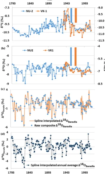
The stable carbon and oxygen isotope compositions (expressed asδ¹³C and δ¹⁸O values in ‰ relative to V-PDB) presented in this paper were derived from two stalagmites (VK1 and NU2; Fig. 1a) from the Baradla Cave (NE Hun- gary; 48^◦28⁰N, 20^◦30⁰E). Despite being 500 m apart in the cave, the two slow-growing speleothems show a clear sim- ilarity in growth rates (VK1: 0.37 and NU2: 0.32 mm yr⁻¹; Fig. 9 in Demény et al., 2017) based on lamina counting and pattern in stable isotope variability. The values, for VK1 and NU2, respectively (Demény et al., 2017), are as follows:

– δ¹³C: median,−10.47 and−9.97; range, 2.16 and 3.15;

SD, 0.53 and 0.64.

– δ¹⁸O: median,−6.86 and−7.41; range, 1.69 and 2.39;

SD, 0.4 and 0.43.

This is not surprising, since the rock cover above the two sample locations is comparable (100–150 m). Both deposits were seasonally laminated, providing a relative chronology of annual accuracy. Besides age estimation based on lamina counting,¹⁴C activity was determined in the selected stalagmites. Radiocarbon measurements clearly reflected the post- 1950 elevated atmospheric signal. Thus, the best match was obtained by shifting the NU2 and VK1 records by 3 and 5 years, respectively (Demény et al., 2017), supporting the synchronization of the individual isotope records. The good match of the isotopic peaks and the similarδ¹³C (Fig. 1a) andδ¹⁸O (Fig. 1b) amplitudes both argue for comparable water storage time in the feeding karst water system. Based on lamina counting, the chronological error at the base of VK1 is estimated to be between 3 and 5 years. However,

(3)

the perfect matches found for δ¹³C (see Fig. 1a) andδ¹⁸O (see Fig. 1b) suggest that the chronological difference is much smaller. Moreover, the stable isotope records of the two stalagmites complement one another by filling the hiatuses found (Fig. 1a). To construct composite isotope records from the two stalagmites’δ¹³C andδ¹⁸O records, the original raw data were normalized using mean and standard deviation for the 1950–2000 period (an interval of simultaneous growth for the VK1 and NU2 stalagmites) and merged to a common timescale to provide a regional reference (Demény et al., 2017). Hereinafter, the composite records are expressed as1¹³CBaradlaand1¹⁸OBaradla.

To test the skill of the methodology, the relationship of climate, and the processed evenly spaced 1¹³CBaradla and 1¹⁸OBaradla products was assessed. Thus, monthly averages of temperature and monthly precipitation totals corresponding to the cave location were retrieved a global gridded climate dataset (CRU TS3.23; Harris et al., 2014) with a time span covering 1901–2014 and a grid space of 0.5^◦.

2.2 Methodology

2.2.1 Interpolation and resampling with spectral guidance

To achieve a regular time axis, the gaps in the 1¹³C_Baradla and1¹⁸OBaradlatime series were filled by cubic spline fitting, and resampled to an annual resolution by averaging (Fig. 1) (De Boor, 1978) in an R statistical environment (R Core Team, 2016) using thestringrpackage (Wickham, 2015) and the spline function of thestatspackage (R Core Team, 2016).

The advantages of cubic spline fitting are that it is considered to be highly effective in the preservation of the spectral characteristics of the original record (Horowitz, 1974);

it is robust and computationally efficient, thus being suitable to process large data sets (Musial et al., 2011); it out- performs linear interpolation – especially in the higher frequency domain (Schulz and Stattegger, 1997); and it has a smaller chance of overfitting as a higher-order spline.

Furthermore, spline interpolation does not introduce outliers as the Lomb–Scargle reconstruction (Hocke and Kämpfer, 2009) or the Kondrashov and Ghil technique (Kon- drashov and Ghil, 2006) do when missing values are – for example – seasonally clustered, thus rendering the estimation of ranges of frequencies and the power spectrum unreliable (Musial et al., 2011). However, because of its “local” estimation characteristic (i.e., lack of predictive capacity), with the increase in a prolonged gap the accuracy of spline interpolation decreases. With the use of rigorous tests it has been documented that if the length of the gap is, for example, slightly above 10 % of the total data length, the mean absolute error of the estimation will be below 0.1. In the case of the Baradla composite stable isotope records, the maximum gap length was 4.85 years, corresponding to 2.24 %, mean-

Figure 1.Rawδ¹³C(a)andδ¹⁸O(b)records of the NU2 and VK1 speleothems (hiatuses indicated by gaps in the line), cubic spline fitted to the(c)original unevenly spaced1¹⁸O_Baradla time series and the(d)annual averages derived from the interpolated time series. The blue and orange rectangles in panels(a, b)mark the hiatuses of the NU2 and VK1 speleothems, respectively, as discussed in Demény et al. (2017).

ing that the use of spline interpolation could be suggested in opposition to the previously mentioned methods. For further details on the benefits and drawbacks of the previously mentioned methods and the detailed documentation on the effects of gap length on mean absolute error the reader is referred to Musial et al. (2011).

It should also be noted that in the case of interpolation, regardless of the method applied, the high-frequency com- ponents in the spectrum will be underestimated; thus the interpolated time series will become “reddened” (Schulz and Stattegger, 1997).

(4)

Therefore, the spectral bias caused by interpolation has to be objectively quantified and checked. The spectral characteristics of the original and the interpolated data have to be compared to detect potential spectral artifacts. Thus, a threshold frequency is needed to be quantified, beyond which (i) the interpolation (cubic spline in the present case) leaves the original spectrum mainly unchanged, and (ii) the significant powers of the original time series are in coherence with the interpolated spectrum.

To determine this threshold frequency objectively, first the spectral characteristics of the original and the interpolated time series were explored to see if the powers of the time series’ Lomb–Scargle–Fourier transform periodograms (LSPs) (Lomb, 1976; Scargle, 1982) are significant against red- noise background from a first-order autoregressive (AR(1)) process using REDFIT (Schulz and Mudelsee, 2002). In the calculations, aWelch Iwindow with two overlapping (50 %) segments was used, the oversampling parameter was set as ofac=4, as in the works of Hocke and Kämpfer (2009) and Press et al. (1996), and hifac=1, the number of Monte Carlo simulations to obtain the significance levels was nsim=1000, in line with other studies dealing with speleothem time series (Holzkämper et al., 2004; Neff et al., 2001), and the red-noise boundary was estimated as the bias-corrected 80 % chi-squared limit of a fitted AR(1) process. For the computations, the redfitfunction of the dplR package was used (Bunn, 2008). The obtained periodograms will be referred to hereinafter as redfit Lomb–

Scargle–Fourier transform periodograms (rLSPs). The obtained rLSPs of the original and the interpolated time series were then compared visually.

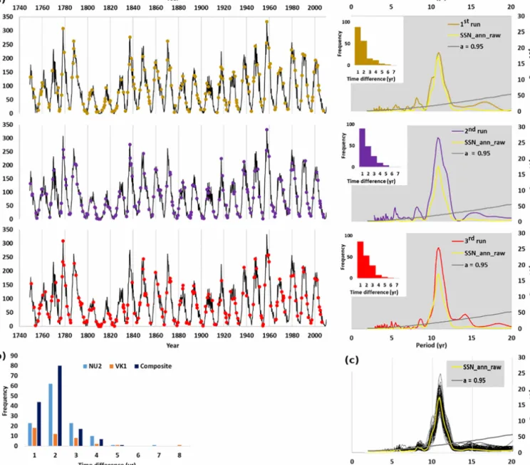
A record with pronounced periodic signals was selected to test the performance and robustness of the presented approach. Seasonal averages were computed from the monthly mean total sunspot numbers (SSN; WDC SILSO, 2017) and randomly resampled. Seven data points were taken randomly from each block of 10 years to replicate the resolution of the Baradla speleothem (avg. 0.7 stable isotope data per year).

This was repeated a 100 times, so an ensemble of 100 randomly resampled time series were obtained, replicating the nonuniform resolution of the Baradlaδ¹⁸O record. The maximum difference between the consecutive samples in the arti- ficially resampled dataset was practically the same as in that in the Baradla speleothem record (∼7; Fig. 2a, b). Moreover, the relatively large gaps (≥4 year) represented about 5–10 % of the artificial time series, which was in harmony with the original speleothem (raw and composite) record (Fig. 2b).

The only slight difference between the speleothem record and the artificial time series was seen in the most frequent gaps. In the case of the VK1 record, the most frequent gap between two samples was the same as in the artificial time series – 1 year – while in one of the raw speleothems and the composite record, this was 2 years.

As a final step in line with the proposed protocol, the 100 randomly resampled time series were spline-interpolated and

annual averages were calculated, and these were then processed using REDFIT to assess their spectral characteristics and compare them to the spectra of the actual annual averages of the original (sunspot) record.

All the 100 rLSPs replicated the well-known∼11-year sunspot cycle (α=0.95). Moreover, most of the rLSPs of the unequally spaced artificial time series mirrored an even smaller peak (∼8 years). However, the noise caused by spline interpolation can be clearly observed at the higher frequencies (Fig. 2c), highlighting the necessity of control- ling/checking the spectral bias caused by interpolation.

After the visual comparison of the rLSPs, the coherence of the unevenly spaced original and the interpolated time series was also computed, using REDFIT-X (Björg Ólafsdóttir et al., 2016), developed for the cross-spectral analysis of unevenly spaced paleoclimate time series. The run parameters were the same as those indicated above.

Combining the visual comparison of the original and interpolated time series’ rLSPs with their quantified coherence spectrum, the smallest significant period of the original data was determined, which was also present, and in coherence with the spline-interpolated one. This could then be set as the threshold frequency above which the original spectra could be taken as unbiased. Finally, the variance below this threshold frequency was removed/filtered from the spline- interpolated time series using the bandpass function of the astrochron package (Meyers, 2014).

2.2.2 Wavelet transform coherence

Data preprocessing was necessary to ensure a time series is evenly spaced in time (Sect. 2.2.1) in order to find the areas with common powers between the speleothem stable isotope time series and the climatic data in the time–frequency space.

Wavelet transform coherence (WTC) (Torrence and Webster, 1999) was used to assess and visualize the coherence and phase-angle difference of the time series on so-called power spectrum density (PSD) graphs (e.g., Fig. 4). The phase- angle differences are indicated by arrows. It should be noted that, depending on the chronological error, the phase information can be biased. For example, an error of 4 years could already reverse the phase angle of an 8-year period signal.

Thus, keeping the chronological error of the input data (see Sect. 2.1) in mind, to avoid over-interpretation, only the dominantly in-phase relationships (indicated by arrows pointing to the right) and dominantly anti-phase relationships (arrows pointing to the left) are considered in the study.

WTC may be considered similar to a correlation coeffi- cient, but with the difference that here we are dealing with a localized time–frequency space (Grinsted et al., 2004). It is based on wavelet spectrum analysis, a function localized in both frequency and time, with a mean of zero (Grinsted et al., 2004), and may be taken as the convolution of the data and the wavelet function (Kovács et al., 2010) for a time series (X_n,n=1, . . . , N) with a1tdegree of uniform resolu-

(5)

Figure 2.Illustration of the performance and robustness of the resampling protocol.(a)Three examples of the randomly resampled annual mean sunspot numbers (left panels), along with the histograms representing the distribution of time differences between the resampled values, and the rLSPs of the original and the corresponding resampled annual mean sunspot number data (right panels).(b)Histograms of the time differences between the Baradla stable isotope records’ samples.(c)The rLSPs of the original and the 100 randomly resampled annual mean sunspot number data. The rLSP of the annual mean sunspot numbers is in yellow (right column inaandc). The rLSPs of the randomly resampled un-evenly spaced artificial (sunspot) time series, spline interpolated and annualized from the monthly mean sunspot numbers are in orange, purple and red for the three examples respectively(a), and in black for all the 100 randomly resampled time series(c). The bias-corrected 95 % chi-squared limit of a fitted AR(1) process for the rLSPs is shown in grey(a, c).

tion Eq. (1):

W_n^X(s)= r1t

S XN

n⁰=1X_n⁰9^∗

n⁰−n1t S

, (1)

whereN is the length of the time series,ψ^∗ is the wavelet function, andsis the scale. In this study the Morlet mother wavelet (Morlet et al., 1982) was used to generate daugh- ter wavelets, because it establishes a clear distinction be-

tween random fluctuations and periodic regions (Andreo et al., 2006).

If two time series correlate, it does not mean that their WTC will indicate a strong common periodic behavior, because the periodic component has to be present in order to find a meaningful WTC. In the course of the evaluation only those signals were considered which were significant (α=0.1) against an AR(1) process; for details see Roesch

(6)

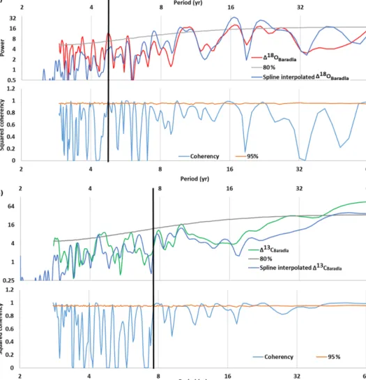
Figure 3. rLSPs (upper panels) and coherency spectra (lower panels) of the original, and the spline-interpolated (a)1¹⁸O_Baradla and (b)1¹³C_Baradla records of the Baradla speleothem. The bias-corrected 80% chi-squared limit of a fitted AR(1) process for the rLSPs is shown in grey. The coherency spectra were produced with a 95 % Monte Carlo false-alarm levels (lower panels). The vertical black line indicates the determined cut-off period.

and Schmidbauer (2014). Since the wavelet functions are normalized to have unit energy, the obtained wavelet trans- forms may even be compared with other time series (Tor- rence and Compo, 1998).

From a practical point of view, the PSD graphs of the WTC analysis between the stable isotope time series and the monthly climate data were calculated to find the months with the highest response. Then the monthly data which indicated the strongest coherence were averaged (e.g., December–

January–February–March) and their WTC with the proxy time series was calculated again. Even if there was a month in between those indicating a strong relationship with the climate data (e.g., strong relationship with December and February–March; weak relationship with January), the multi- monthly averages (December–March and February–March) were calculated and assessed using WTC. Thus, consecutive multi-monthly averages (seasons) were obtained, indicating the maximum response forming the final output of

the analysis. The WTC PSD graphs were generated with the analyze.coherencyfunction of theWavelet-comp package (Roesch and Schmidbauer, 2014) inR.

3 Results and discussions

3.1 Data preprocessing before WTC analysis

After obtaining the rLSPs and the coherency spectra of the original and spline-interpolated1¹³C_Baradlaand1¹⁸O_Baradla time series, these were compared as discussed in Sect. 2.2.1.

As low as a period of ∼5 years, the significant powers (α=0.8) of the original 1¹⁸O_Baradla record were all mirrored in the spline-interpolated one, and to a high degree of coherency, and the original, and the interpolated record indicated a similar pattern on their rLSPs (Fig. 3a). However, around and below the 4.5-year period, the significant powers of the original1¹⁸O_Baradla record were no longer reflected

(7)

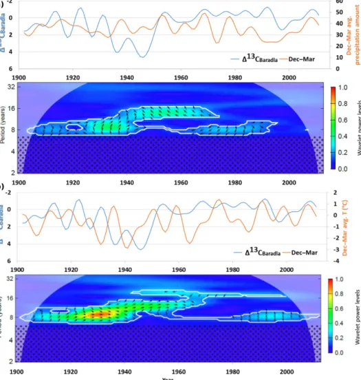
Figure 4.Time series of the 7.5-year low-passed composite1¹³C_Baradla records (on a reversed axis) with the gridded December–March average(a)temperature and(b)precipitation amount (Harris et al., 2014) (upper panel) and their time–frequency coherency image (lower panel). The white contours in the lower panel show the 90 % confidence levels calculated based on 1000 AR(1) surrogates. The black arrows indicate the phase-angle difference, where an in-phase relationship is indicated by arrows pointing to the right, whereas anti-phase relationship is shown by arrows pointing to the left. The dotted area marks the period band below the cut-off threshold.

in the spline-interpolated one, and the two time series’ level of coherency became generally low as well. Therefore, to be consistent and to take a conservative (that is, careful) approach, the period domain below 4.5 years was omitted with a low-pass filter for the1¹⁸O_Baradlatime series. It should be noted, however, that in cases when the storage component in the aquifer is larger than the numerically chosen cut-off period, the water storage time in the karst may amplify the auto-correlation of the isotopic time series.

The same steps were then performed on the 1¹³CBaradla

record as well. Thus, around and below the ∼7.5-year period, the significant powers of the original1¹³C_Baradlarecord were no longer reflected in the spline-interpolated one, and the level of the two time series’ coherency became generally low as well. Above the threshold, the avg. squared coherency is 0.9 and only drops below 0.8 in exceptional cases, while below it, its average is 0.57 and frequently drops to

zero (Fig. 3b). Thus, the domain below 7.5 years was cut off from the1¹³C_Baradla spectrum to avoid the spectral bias caused by spline interpolation (Fig. 3b).

3.2 Climate signals in the stable isotope composition of carbonates of the Baradla speleothems

To present the applicability of the now equally spaced paleoproxy data in climate studies, the 1¹³C_Baradla and 1¹⁸O_Baradlarecords were compared to precipitation and temperature (primary climate variables).

The first step was to explore whether meaningful and significant coherences could be found in the time–frequency space between the equally spaced and 7.5-year low-passed speleothem 1¹³C_Baradla time series and similarly low- passed primary climate parameters (precipitation, temperature; Fig. 4). In the case of the composite1¹³C_Baradlarecord,

(8)

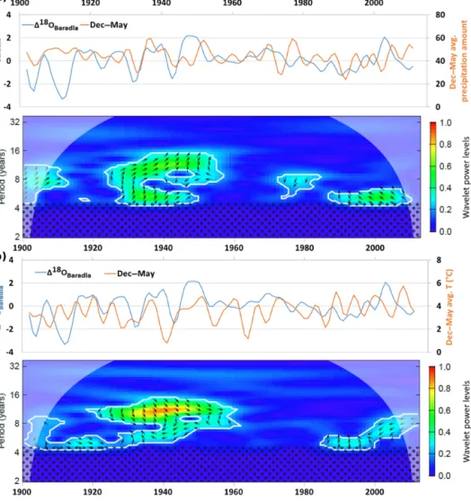
Figure 5.Time series of the 4.5-year low-passed composite1¹⁸O records with the gridded climate data (Harris et al., 2014) December–May average(a)precipitation and(b)temperature (upper panels) and their time–frequency coherency image (lower panels). For further details see the caption of Fig. 4.

the best coherence was found with the December–March averages of temperature and precipitation amount, although a more persistent relationship was detected with precipitation than with temperature (Fig. 4).

The generally anti-phase coherence/relationship between precipitation amount and the1¹³CBaradlarecord is in accor- dance with the former interpretation (Demény et al., 2017), namely that a higher amount of precipitation results in en- hanced biological soil activity, more biogenic CO₂ in the soil, and consequently more negative 1¹³C values in the speleothems of the Baradla Cave. Although the relationship between the1¹³C and precipitation amount had previously been observed for individual records using visual compar- isons and regression analysis (Demény et al., 2017), it was found to be weak due to dating uncertainties and the varying effect of additional factors contributing to the precipitation–

sedimentary proxy relationship (e.g., kinetic fractionation, vegetation change, prior calcite precipitation; see Fairchild

and Baker, 2012, for the compilation of governing factors).

Nevertheless, with WTC analysis, it was not the whole spectra which was taken into account all at once (as in the case of linear regression analysis), but the relationship was mapped for each frequency band and observed over time. The phase of the coherence was observed to vary on the decadal scale. A generally anti-phase difference was revealed between1¹³C and precipitation amount (Fig. 4a).

As for the relationship between 1¹³C and temperature, significant coherences were observed in the 8–16-year period band, but these, however, weakened between ∼1960 and

∼1975. Furthermore, the phase-angle differences were not persistent afterwards (Fig. 4b). The varying coherence with temperature – regarding the period and phase angle (Fig. 4b) – might be related to biological activity in the soil driven primarily by the interplay between temperature and water sat- uration conditions mutually affecting the decomposition of

(9)

the organic matter that is the dominant source of speleothem carbon (Noronha et al., 2015).

Significant coherences were found between the Baradla speleothem’s 1¹⁸O_Baradla records and the multi-monthly (December–May) averages of precipitation and temperature.

The coherence between precipitation and 1¹⁸O_Baradla was patchily developed, and was significant in the intervals 1900 to ∼1915 and ∼1920 to ∼1955 for the period range of 4–16 years, and between ∼1970 and 2010 for around the

∼5-year period (Fig. 5a). In the case of temperature and 1¹⁸O_Baradlaa more developed, less patchy pattern was seen, with one longer period lacking coherence between ∼1960 and the early 1980s (Fig. 5b). Coherence is primarily present in the 4–16-year period range, as in the previous case. A mutual characteristic of the relationship of both precipitation and temperature to1¹⁸OBaradla is the common discon- tinuity around the 1960s (Fig. 5). Such coherences were to be expected, since the oxygen isotope composition of the speleothem is driven by temperature and drip water composition (Lachniet, 2009). Drip water composition is directly related to meteoric water composition, governed by atmospheric temperature and moisture origin in the mid-latitudes (Dansgaard, 1964), and has been documented in the sur- roundings of the study area (Bottyán et al., 2017; Kaiser et al., 2001). In relation to the seasonal characteristic of the response, a strong contrast exists in the seasonal water balance at the Baradla Cave. Precipitation exceeds evapotranspiration from October to April (Demény et al., 2017), which is well reflected in the isotopic character of the drip water, arguing for the overwhelming dominance (∼90%) of winter precipitation (Czuppon et al., 2018). Large-scale tropospheric circulation controls precipitation amount and water stable isotope composition over Europe (Comas-Bru et al., 2016), which invites future investigations of coherence with atmospheric circulation indices.

However, with regard to the phase differences between the1¹⁸O_Baradlarecords and the climate parameters, a some- what confusing picture can be observed in the investigated

∼110 years. The phase-angle differences changed multiple times, and a dominant direction could hardly be assigned.

This may be a result of the complex interplay of governing factors.

4 Data availability

The data sets produced with the methodology presented in the paper are available at https://doi.org/10.1594/PANGAEA.875917.

5 Conclusions

A cubic-spline-based universally applicable methodology was developed to handle the uneven spacing of sedimentary proxy records. Additionally, the bias that interpolation may

cause was evaluated with spectral control. The methodology was successfully applied to the composite stable carbon and oxygen isotope records of the speleothems of the Baradla Cave, NE Hungary. The composite stable isotope records of the Baradla Cave speleothem were compared with temperature and precipitation-amount data at a monthly resolution using wavelet transform coherence analyses. A generally negative relationship between the carbon isotope record and cold season precipitation amount was revealed, in accor- dance with earlier assumptions. With temperature, however, a less persistent relationship was observed, and this is sus- pected to be related to biological activity in the soil. In the case of oxygen isotopic composition, its relationship with temperature and precipitation amount was less clear, proba- bly due to the competing and/or superimposed factors deter- mining the carbonate’s oxygen isotopic composition. These observations provide a firm basis for the interpretation of stable isotope data obtained for the Baradla Cave system.

The now evenly resampled and low-pass-filtered composite records may also serve as regional benchmarks in future proxy paleoclimate evaluations.

Author contributions. IGH developed the model code and performed the simulations. ZK preprocessed the data and provided the composite records. AD conceived the study and provided the geochemical interpretation. SL- ˝O was responsible for the cave studies.

All authors took part in the manuscript preparation.

Competing interests. The authors declare that they have no con- flict of interest.

Acknowledgements. Financial support was received from the Hungarian Academy of Sciences (MTA “Lendület” program;

LP2012-27/2012), the National Research, Development and Innovation Office (OTKA NK 101664), and the János Bolyai Research Scholarship of the Hungarian Academy of Sciences. This is contribution no. 53 of the 2ka Palæoclimatology Research Group.

Edited by: David Carlson

Reviewed by: Laia Comas-Bru and one anonymous referee

References

Andreo, B., Jiménez, P., Durán, J. J., Carrasco, F., Vadillo, I., and Mangin, A.: Climatic and hydrological variations during the last 117–166 years in the south of the Iberian Peninsula, from spectral and correlation analyses and continuous wavelet analyses, J. Hy- drol., 324, 24–39, https://doi.org/10.1016/j.jhydrol.2005.09.010, 2006.

Baker, A. and Bradley, C.: Modern stalagmiteδ¹⁸O: Instrumental calibration and forward modelling, Global Planet. Change, 71, 201–206, https://doi.org/10.1016/j.gloplacha.2009.05.002, 2010.

(10)

Baker, A., C. Hellstrom, J., Kelly, B. F. J., Mariethoz, G., and Trouet, V.: A composite annual-resolution stalagmite record of North Atlantic climate over the last three millennia, Sci. Rep.- UK, 5, 10307, https://doi.org/10.1038/srep10307, 2015.

Björg Ólafsdóttir, K., Schulz, M., and Mudelsee, M.:

REDFIT-X: Cross-spectral analysis of unevenly spaced paleoclimate time series, Comput. Geosci., 91, 11–18, https://doi.org/10.1016/j.cageo.2016.03.001, 2016.

Bottyán, E., Czuppon, G., Weidinger, T., Haszpra, L., and Kármán, K.: Moisture source diagnostics and isotope characteristics for precipitation in east Hungary: implications for their relationship, Hydrolog. Sci. J., 62, 2049–2060, https://doi.org/10.1080/02626667.2017.1358450, 2017.

Breitenbach, S. F. M., Lechleitner, F. A., Meyer, H., Diengdoh, G., Mattey, D., and Marwan, N.: Cave ventilation and rainfall signals in dripwater in a monsoonal setting – a monitoring study from NE India, Chem. Geol., 402, 111–124, https://doi.org/10.1016/j.chemgeo.2015.03.011, 2015.

Bunn, A. G.: A dendrochronology program library in R (dplR), Dendrochronologia, 26, 115–124, https://doi.org/10.1016/j.dendro.2008.01.002, 2008.

Comas-Bru, L., McDermott, F., and Werner, M.: The effect of the East Atlantic pattern on the precipitation δ¹⁸O–

NAO relationship in Europe, Clim. Dynam., 47, 2059–2069, https://doi.org/10.1007/s00382-015-2950-1, 2016.

Cosford, J., Qing, H., Eglington, B., Mattey, D., Yuan, D., Zhang, M., and Cheng, H.: East Asian monsoon variability since the Mid-Holocene recorded in a high-resolution, absolute-dated aragonite speleothem from eastern China, Earth Planet. Sc. Lett., 275, 296–307, https://doi.org/10.1016/j.epsl.2008.08.018, 2008.

Czuppon, G., Demény, A., Leél- ˝Ossy, S., Óvari, M., Mol- nár, M., Stieber, J., Kiss, K., Kármán, K., Surányi, G., and Haszpra, L.: Cave monitoring in the Béke and Baradla caves (Northeastern Hungary): implications for the conditions for the formation cave carbonates, Int. J. Speleol., 47, 13–28, https://doi.org/10.5038/1827-806X.47.1.2110, 2018.

Dansgaard, W.: Stable isotopes in precipitation, Tellus, 16, 436–

468, 1964.

De Boor, C.: A Practical Guide to Splines, Springer-Verlag, New York, 1978.

Deininger, M., McDermott, F., Mudelsee, M., Werner, M., Frank, N., and Mangini, A.: Coherency of late Holocene European speleothem δ¹⁸O records linked to North At- lantic Ocean circulation, Clim. Dynam., 49, 595–618, https://doi.org/10.1007/s00382-016-3360-8, 2017.

Demény, A., Németh, A., Kern, Z., Czuppon, G., Molnár, M., Leél- Ossy, S., Óvári, M., and Stieber, J.: Recently forming stalag-˝ mites from the Baradla Cave and their suitability assessment for climate–proxy relationships, Central European Geology, 60, 1–

34, https://doi.org/10.1556/24.60.2017.001, 2017.

Duan, F., Wang, Y., Shen, C.-C., Wang, Y., Cheng, H., Wu, C.-C., Hu, H.-M., Kong, X., Liu, D., and Zhao, K.: Ev- idence for solar cycles in a late Holocene speleothem record from Dongge Cave, China, Sci. Rep.-UK, 4, 5159, https://doi.org/10.1038/srep05159, 2014.

Ersek, V., Clark, P. U., Mix, A. C., Cheng, H., and Lawrence Edwards, R.: Holocene winter climate variability in mid- latitude western North America, Nat. Commun., 3, 1219, https://doi.org/10.1038/ncomms2222, 2012.

Fairchild, I. J. and Baker, A.: Geochemistry of Speleothems, in: Speleothem Science: From Process to Past Envi- ronments, John Wiley & Sons, Ltd, Chichester, UK, https://doi.org/10.1002/9781444361094.ch8, 2012.

Fairchild, I. J. and Treble, P. C.: Trace elements in speleothems as recorders of environmental change, Quaternary Sci. Rev., 28, 449–468, https://doi.org/10.1016/j.quascirev.2008.11.007, 2009.

Grinsted, A., Moore, J. C., and Jevrejeva, S.: Application of the cross wavelet transform and wavelet coherence to geophysical time series, Nonlin. Processes Geophys., 11, 561–566, https://doi.org/10.5194/npg-11-561-2004, 2004.

Hammer, Ø.: PAST – PAleontological STatistics, Version 3.15, Nat- ural History Museum, University of Oslo, Oslo, Norway, 2017.

Harris, I., Jones, P. D., Osborn, T. J., and Lister, D. H.: Up- dated high-resolution grids of monthly climatic observations – the CRU TS3.10 Dataset, Int. J. Climatol., 34, 623–642, https://doi.org/10.1002/joc.3711, 2014.

Hocke, K. and Kämpfer, N.: Gap filling and noise reduc- tion of unevenly sampled data by means of the Lomb- Scargle periodogram, Atmos. Chem. Phys., 9, 4197–4206, https://doi.org/10.5194/acp-9-4197-2009, 2009.

Holmgren, K., Lee-Thorp, J. A., Cooper, G. R. J., Lundblad, K., Par- tridge, T. C., Scott, L., Sithaldeen, R., Siep Talma, A., and Tyson, P. D.: Persistent millennial-scale climatic variability over the past 25,000 years in Southern Africa, Quaternary Sci. Rev., 22, 2311–

2326, https://doi.org/10.1016/S0277-3791(03)00204-X, 2003.

Holzkämper, S., Mangini, A., Spötl, C., and Mudelsee, M.: Tim- ing and progression of the Last Interglacial derived from a high alpine stalagmite, Geophys. Res. Lett., 31, L07201, https://doi.org/10.1029/2003GL019112, 2004.

Horowitz, L.: The effects of spline interpolation on power spectral density, IEEE T. Acoust. Speech, 22, 22–27, 1974.

Jex, C. N., Baker, A., Fairchild, I. J., Eastwood, W. J., Leng, M. J., Sloane, H. J., Thomas, L., and Bekaro˘glu, E.:

Calibration of speleothem δ¹⁸O with instrumental climate records from Turkey, Global Planet. Change, 71, 207–217, https://doi.org/10.1016/j.gloplacha.2009.08.004, 2010.

Kaiser, A., Scheifinger, H., Kralik, M., Papesch, W., Rank, D., and Stichler, W.: Links between meteorological conditions and spa- tial/temporal variations in long-term isotope records from the Austrian precipitation network, Study of environmental change using isotope techniques, International Atomic Energy Agency (IAEA), IAEA-CSP–13/P, 67–77, 2001.

Kondrashov, D. and Ghil, M.: Spatio-temporal filling of missing points in geophysical data sets, Nonlin. Processes Geophys., 13, 151–159, https://doi.org/10.5194/npg-13-151-2006, 2006.

Kovács, J., Hatvani, I. G., Korponai, J., and Kovács, I. S.: Morlet wavelet and autocorrelation analysis of long-term data series of the Kis-Balaton water protection system (KBWPS), Ecol. Eng., 36, 1469–1477, https://doi.org/10.1016/j.ecoleng.2010.06.028, 2010.

Lachniet, M. S.: Climatic and environmental controls on speleothem oxygen-isotope values, Quaternary Sci. Rev., 28, 412–432, https://doi.org/10.1016/j.quascirev.2008.10.021, 2009.

Lachniet, M. S., Burns, S. J., Piperno, D. R., Asmerom, Y., Polyak, V. J., Moy, C. M., and Christenson, K.: A 1500-year El Niño/Southern Oscillation and rainfall history for the Isthmus of Panama from speleothem calcite, J. Geophys. Res., 109, D20117, https://doi.org/10.1029/2004JD004694, 2004.

(11)

Lomb, N. R.: Least-squares frequency analysis of unequally spaced data, Astrophys. Space Sci., 39, 447–462, 1976.

Mattey, D., Lowry, D., Duffet, J., Fisher, R., Hodge, E., and Frisia, S.: A 53 year seasonally resolved oxygen and carbon isotope record from a modern Gibraltar speleothem: Reconstructed drip water and relationship to local precipitation, Earth Planet.

Sc. Lett., 269, 80–95, https://doi.org/10.1016/j.epsl.2008.01.051, 2008.

Mattey, D. P., Atkinson, T. C., Barker, J. A., Fisher, R., Latin, J. P., Durrell, R., and Ainsworth, M.: Carbon dioxide, ground air and carbon cycling in Gibraltar karst, Geochim. Cosmochim. Ac., 184, 88–113, https://doi.org/10.1016/j.gca.2016.01.041, 2016.

McCabe-Glynn, S., Johnson, K. R., Strong, C., Berkelham- mer, M., Sinha, A., Cheng, H., and Edwards, R. L.: Vari- able North Pacific influence on drought in southwestern North America since AD 854, Nat. Geosci., 6, 617–621, https://doi.org/10.1038/ngeo1862, 2013.

Meyers, S. R.: astrochron: An R Package for Astrochronology, available at: https://cran.r-project.org/package=astrochron (last access: January 2018), 2017.

Morlet, J., Arens, G., Fourgeau, E., and Giard, D.: Wave prop- agation and sampling theory; Part I, Complex signal and scattering in multilayered media, Geophysics, 47, 203–221, https://doi.org/10.1190/1.1441328, 1982.

Mudelsee, M.: Climate Time Series Analysis: Classical Statistical and Bootstrap Methods, Springer, Dordecht, 2010.

Musial, J. P., Verstraete, M. M., and Gobron, N.: Technical Note: Comparing the effectiveness of recent algorithms to fill and smooth incomplete and noisy time series, Atmos.

Chem. Phys., 11, 7905–7923, https://doi.org/10.5194/acp-11- 7905-2011, 2011.

Neff, U., Burns, S. J., Mangini, A., Mudelsee, M., Fleitmann, D., and Matter, A.: Strong coherence between solar variability and the monsoon in Oman between 9 and 6 kyr ago, Nature, 411, 290–293, https://doi.org/10.1038/35077048, 2001.

Noronha, A. L., Johnson, K. R., Southon, J. R., Hu, C., Ruan, J., and McCabe-Glynn, S.: Radiocarbon evidence for decomposition of aged organic matter in the vadose zone as the main source of speleothem carbon, Quaternary Sci. Rev., 127, 37–47, https://doi.org/10.1016/j.quascirev.2015.05.021, 2015.

Press, W. H., Teukolsky, S. A., Vetterling, W. T., and Flannery, B. P.:

Numerical recipes in C, Cambridge University Press, Cambridge, UK, 1996.

R Core Team: R: A Language and Environment for Statistical Com- puting, R Foundation for Statistical Computing, Vienna, Austria, 2016.

Riechelmann, D. F. C., Schröder-Ritzrau, A., Scholz, D., Fohlmeis- ter, J., Spötl, C., Richter, D. K., and Mangini, A.: Monitoring Bunker Cave (NW Germany): A prerequisite to interpret geochemical proxy data of speleothems from this site, J. Hydrol., 409, 682–695, https://doi.org/10.1016/j.jhydrol.2011.08.068, 2011.

Roberts, J., Curran, M., Poynter, S., Moy, A., Ommen, T. v., Vance, T., Tozer, C., Graham, F. S., Young, D. A., Plummer, C., Pedro, J., Blankenship, D., and Siegert, M.: Correlation confidence limits for unevenly sampled data, Comput. Geosci., 104, 120–124, https://doi.org/10.1016/j.cageo.2016.09.011, 2017.

Roesch, A. and Schmidbauer, H.: WaveletComp: A guided tour through the R-package, available at: http://www.hs-stat.com/

projects/WaveletComp/WaveletComp_guided_tour.pdf (last access: January 2018), 2014.

Scargle, J. D.: Studies in astronomical time series analysis. II- Statistical aspects of spectral analysis of unevenly spaced data, Astrophys. J., 263, 835–853, 1982.

Schulz, M. and Mudelsee, M.: REDFIT: estimating red-noise spectra directly from unevenly spaced paleoclimatic time series, Comput. Geosci., 28, 421–426, https://doi.org/10.1016/S0098- 3004(01)00044-9, 2002.

Schulz, M. and Stattegger, K.: Spectrum: spectral analysis of unevenly spaced paleoclimatic time series, Comput. Geosci., 23, 929–945, https://doi.org/10.1016/S0098-3004(97)00087-3, 1997.

Schulz, M., Berger, W. H., Sarnthein, M., and Grootes, P. M.:

Amplitude variations of 1470-year climate oscillations during the last 100,000 years linked to fluctuations of continental ice mass, Geophys. Res. Lett., 26, 3385–3388, https://doi.org/10.1029/1999GL006069, 1999.

Surić, M., Lonˇcarić, R., Boˇcić, N., Lonˇcar, N., and Buzjak, N.: Monitoring of selected caves as a prerequisite for the speleothem-based reconstruction of the Quaternary environment in Croatia, Quatern. Int., https://doi.org/10.1016/j.quaint.2017.06.042, in press, 2018.

Torrence, C. and Compo, G. P.: A Practical Guide to Wavelet Analysis, B. Am. Meteo- rol. Soc., 79, 61–78, https://doi.org/10.1175/1520- 0477(1998)079<0061:APGTWA>2.0.CO;2, 1998.

Torrence, C. and Webster, P. J.: Interdecadal Changes in the ENSO–Monsoon System, J. Cli- mate, 12, 2679–2690, https://doi.org/10.1175/1520- 0442(1999)012<2679:ICITEM>2.0.CO;2, 1999.

von Gunten, L., D’Andrea, W. J., Bradley, R. S., and Huang, Y.:

Proxy-to-proxy calibration: Increasing the temporal resolution of quantitative climate reconstructions, Sci. Rep.-UK, 2, 609, https://doi.org/10.1038/srep00609, 2012.

Wackerbarth, A., Langebroek, P. M., Werner, M., Lohmann, G., Riechelmann, S., Borsato, A., and Mangini, A.: Sim- ulated oxygen isotopes in cave drip water and speleothem calcite in European caves, Clim. Past, 8, 1781–1799, https://doi.org/10.5194/cp-8-1781-2012, 2012.

Wassenburg, J. A., Dietrich, S., Fietzke, J., Fohlmeister, J., Jochum, K. P., Scholz, D., Richter, D. K., Sabaoui, A., Spotl, C., Lohmann, G., Andreae, M. O., and Immenhauser, A.: Reorganization of the North Atlantic Oscillation during early Holocene deglaciation, Nat. Geosci., 9, 602–605, https://doi.org/10.1038/ngeo2767, 2016.

Wickham, H.: stringr: Simple, Consistent Wrappers for Com- mon String Operations, R package, available at: https://CRAN.

R-project.org/package=stringr (last access: January 2018), 2017.