DOI:10.28974/idojaras.2019.1.1
IDŐJÁRÁS
Quarterly Journal of the Hungarian Meteorological Service Vol. 123, No. 1, January – March, 2019, pp. 1–18
Estimation of rainfall erosivity in Piedmont (Northwestern Italy) by using 10-minute fixed-interval rainfall data
Fiorella Acquaotta 1,2, Alice Baronetti 1, Mario Bentivenga 3, Simona Fratianni 1,2,*, and Marco Piccarreta 4
1 Dipartimento di Scienze della Terra, Università di Torino, Via Valperga Clauso 35, 10125Torino, Italia
2 NatRisk Centro interdipartimentale sui rischi naturali in ambiente montano e collinare,
Largo Paolo Braccini, 2, 10095, Grugliasco (TO), Italia
3 Dipartimento di Scienze, Università della Basilicata, Viale dell'Ateneo Lucano, 10 - 85100 Potenza, Italia
4 Ministero dell’Istruzione, dell’Università e della Ricerca, Via Giustino Fortunato 8/M, 70125 Bari, Italia
* Corresponding author E-mail: simona.fratianni@unito.it (Manuscript received in final form April 19, 2018)
Abstract⎯ Rainfall erosivity index (EI30) is widely used in soil erosion models for predicting soil loss. This index consists in the product between the maximum intensity of 30-min rainfall and the total kinetic energy of a precipitation event. The main goal of this study was to characterize the soil erosion in Piedmont (Northwestern Italy), studying the magnitude, frequency, and trends of rainfall erosivity. Rainfall erosivity for twelve stations well distributed over the whole region were firstly computed on the basis of 10-min time- resolution rainfall data using a continuous 17-year series of daily rainfall events. For each station the equation to predict EI30 from daily rainfall data was calculated, and, using the Nash and Sutcliffe (1970) model-efficiency, the relationships between real EI30 and modeled EI30 was validated. The rainfall erosivity model was applied to the long term daily rainfall series of the selected stations, to create annual and seasonal erosivity time series for the climate normal period 1986–2015. Afterwards, the Mann–Kendall non-parametric test statistic to detect time trends in the rainfall erosivity time series was applied. The results have led to the conclusion that the annual rainfall erosivity should have experienced mixed trends in most of the study area, although more than half of the stations did not show a statistical trend.
Key-words: rainfall erosivity, time trend, soil erosion, Piedmont, Northwestern Italy
1. Introduction
The concept of soil erosion caused by high energy rainfall was introduced by Hudson (1971) and Wischmeier and Smith (1978) where they describe the erosivity (R) like the interaction between the total kinetic energy of a storm and the soil surface (EI30). Rainfall erosivity is one of the six factors in the Universal Soil Loss Equation, developed to predict the soil erosion (Renard et al., 1997). This equation permits to quantify the ability of rainfall to cause soil loss and is largely used in two of the main prediction models (USLE and RUSLE). The calculation of the erosivity R factor uses breakpoint rainfall intensity data derived from recording rain gauges. Because the limited availability of sub-hourly rainfall data, several study (Ateshian, 1974;
Arnoldus, 1977; Richardson et al., 1983; Bagarello and D’Asaro, 1994; Ferro et al., 1991; Renard and Freimund, 1994; Yu and Rosewell, 1996a, 1996b, 1996c; Loureiro and Couthino, 2001; Yu et al., 2001; Capolongo et al., 2008;
Joon-Hak and Jun-Haeng, 2011) developed methods for the estimation of the EI30 using yearly, monthly and daily rainfall data. Yin et al. (2007) highlighted that the computed R factor will be more accurate with detailed rainfall data.
Richardson et al. (1983), Bagarello et al. (1994), and Petkovsek and Mikoš (2004) tried to predict rainfall erosivity from daily rainfall (P) using the following exponential relationships:
, (1)
where the two Richardson’s coefficients (Richardson et al., 1983) are:
− a, which is considered like the scale factor, and represents the temporal and spatial variability (Richardson et al., 1983);
− b, which is considered as a process parameter and is relatively more constant. The value of the exponent b, obtained by means of theoretically based approach approximates 2.0 (Brown and Foster, 1987), whereas empirical approaches gave values ranging from 1.5 to 2.2 (reference in Bagarello and D’Asoro, 1994; Capolongo et al., 2008).
In recent times, Borrelli et al. (2016) investigated the spatiotemporal distribution of rainfall erosivity in Italy by using both 30- and 60-min time-step data. They have found high variability in erosivity within the country, with a 97% difference between the lowest and highest values. At regional scale relevant studies have been realised especially for such central-southern regions as Basilicata, Calabry, Sicily and Tuscany (D’Asaro et al., 2007; Capolongo et al., 2008; Vallebona et al., 2014; Capra et al., 2017).
For Piedmont (Northwestern Italy), 10-min rainfall records are available from 1989 to 2007. By using data from 12 rain gauges well distributed over the regional territory we tested the Richardson et al. (1983) power relationship between rainfall erosivity (EI30) and daily precipitation > 10 mm (P) to create a newly derived daily erosivity index for each of the investigated stations. It is considered really important due to the lack of a similar study for the region. It has to be stressed that Piedmont is largely devoted to agriculture, in particular to grapevine cultivation, with the production of different top-quality Italian wines. More than 53,000 hectares of the region have been covered by vineyards. According to the agricultural statistical database of the Piedmont Regional Administration, almost 90% of the vineyard surface of the region is on hilly areas and near 2% on mountain areas, which are characterized by large estimates of soil loss due to the high erodibility of the soils and the climate (Tropeano, 1984; Luino, 2005; Corti et al., 2011). On the basis of a recent study of Acquaotta and Fratianni (2013), both the general decreasing trend of precipitation amounts and the weak increasing trend of rainfall intensity occurred in Piedmont from 1971 to 2000 are giving the idea that the erosive power of daily rainfall events in the region should have increased in recent years.
The objective of this study is:
− to quantify principally the rainfall erosivity temporal pattern in the Piedmont region by applying the newly derived daily erosivity rainfall indexes to the climatologic normal 1989–2015 daily record series of the investigated 12 rainfall gauging stations;
− to generate and evaluate extended historical time series of annual rainfall erosivity for the whole region;
− to detect and explain possible time trends in rainfall erosivity.
2. Study area
Piedmont is a region in the northwestern part of Italy (Fig. 1). It borders France and Switzerland, and in Italy it borders the Aosta Valley region, Lombardy, Emilia Romagna, and Liguria. It has an area of 25,402 km2 and is characterized by a complex territory (Fazzini et al., 2004). In fact, the geography is 43%
mountainous, along with extensive areas of hills (30%) and plains (27%). The hills area is composed by Torino, Langhe, and Monferrato. The plain characterized, at East, by the Po Plain crossed by the longest river in Italy, the Po, and its many tributaries. The alpine mountain area is located on the northwestern Italian border with France and Switzerland (Terzago et al., 2012;
Giaccone et al., 2015).
According to the orientation of the Alps and Apennines in Piedmont, there is a strong geographical differentiation in the rainfall distribution, in fact, the annual rainfalls are more abundant along the Alps, in particular at the north, with peaks above 2000 mm/year (Fratianni et al., 2015). While the drier area is the central sector, the Po Plain, with amounts of even less than 600 mm/year in Alessandria plains and Susa valley with the presence of a great number of foehn days (Fratianni et al., 2009).
Acquaotta and Fratianni (2013) have subdivided Piedmont into three different climatic regions on the basis of the Bagnouls and Gaussen’s method:
sub-Mediterranean, temperate and cool-temperate.
The sub-Mediterranean region is located in the Piedmont plain. The region has a subalpine pluviometric regime with a maximum in autumn and spring and a main minimum in winter. The temperate region is characterized by the Piedmont hill, and this area has a prealpine pluviometric regime with a principal maximum in spring and a principal minimum in winter. The cool-temperate region concern the mountain area and has a prealpine pluviometric regime.
Several study developed by the Earth Science Department of Turin show a decrease of consecutive rainy days in the Piedmont plain and hills, a general increase of the annual precipitation, and a positive tendency in the density of precipitation and in the numbers of days. These positive trends make the region particularly prone to severe erosion, with serious consequences on agriculture and grapevine cultivation (Baronetti et al., 2018).
3. Materials and methods 3.1. Database
Rainfall data recorded with a temporal resolution of 10-minute were obtained from twelve electronic rain-gauge stations of the Agenzia Regionale per la Protezione Ambientale (ARPA) operating in Piedmont. The twelve stations (Boves, Bra, Casale Monferrato, Lanzo, Luserna, Mondovì, Oropa, Piamprato, Susa, Torino, Varallo Sesia, and Vercelli) were selected on the basis of their location in order to cover the whole region (Fig. 1) as well as of the quality of the data records, i.e., no missing data (Venema et al., 2013). The system of observation, started in 1986, and we used data until 2015 (Table 1). The rainfall series passed a quality control (Acquaotta et al., 2016; Zandonadi et al., 2016), and for each station an erosive events database has been created (Acquaotta et al., 2018a). The erosive events were determined by the RUSLE criterion (Foster et al., 1981; Renard et al., 1997). A threshold of 1.27 mm (0,05 inch) of precipitation in six hours was selected to represent breaks in rainstorms.
Afterwards, rainstorms with less than 12.7 mm (0.5 inch) of precipitation were omitted from the EI30 calculation. Foster et al. (1981) made an exception for rainstorm events of 15 min duration with at least one peak greater than 6.5 mm.
Recorded rainfall intensities showed different behavior for all the investigated stations confirming the observations made by Acquaotta and Fratianni (2013).
On the whole, 4626 detected storms recorded on a 10-min interval basis were used in the analysis.
Fig. 1. Geographic, location of the meteorological stations in Piedmont, Italy.
Table 1. Characteristics of the meteorological stations analyzed in this study (Latitude North, longitude East, elevation (m ASL))
Stations Latitude N Longitode E Elevation (m) Period
Boves 44° 20' 06'' 7° 33' 43'' 575 1989–2005
Bra 44° 04' 18'' 7° 51' 09'' 285 1993–2007
Casale Monferrato 45° 07' 56'' 8° 30' 15'' 136 1990–2006
Lanzo 45° 17' 23'' 7° 29' 38'' 580 1990–2007
Luserna 44° 48' 46'' 7° 14' 28'' 475 1990–2007
Mondovì 44° 23' 44'' 7° 48' 38'' 422 1993–2007
Oropa 45° 37' 40'' 7° 58' 56'' 1186 1990–2007
Piamprato 45° 33' 02'' 7° 34' 07'' 1550 1993–2007
Susa 45° 08' 31'' 7° 03' 14'' 520 1990–2007
Torino 45° 17' 23'' 7° 41' 23'' 239 1990–2007
Varallo Sesia 45° 49' 14'' 8°16' 30'' 470 1990–2007
Vercelli 45° 19' 32'' 8° 23' 26'' 132 1990–2006
3.2. Rainfall erosivity index
The rainfall erosivity has been calculated by applying the RUSLE R (Renard et al., 1997) equation as proposed by Brown and Foster (1987):
( )
= == n
j m
k k
j
n EI R
1 1
30
1 , (2)
where n is the number of years of records, mj is the number of erosive events of a given year j, and EI30 is the rainfall erosivity index of a singular event k. Thus, the R factor is the average value of the annual cumulative EI30 over a given period. Quantitative evaluation of rainstorm erosivity (EI30) requires rainfall kinetic energy and intensity values associated to 30-minute observation time intervals.
The kinetic energies of all the rainfall events have been evaluated as:
(3)
where E denotes the rainfall kinetic energy in MJ ha-1 mm-1 and Ir is the rainfall intensity in mm h-1. This equation type was tested and found adequate for Mediterranean and Southern European conditions by several authors (Coutinho and Tomas, 1995; Cerro et al., 1998).
The maximum 30 min (0.5 h) intensity, I30 (mm·h− 1), was calculated as:
( )
h I P
5 . 0
30= 30 , (4)
where P30 (mm) was the maximum accumulated rainfall depth in three contiguous 10 min intervals.
The average EI30, as the mean erosivity of all rainfall events, is calculated.
Event rainfall erosivity values (EI) were fitted to the event precipitation amount (P) by the Richardson et al. (1983) exponential relationship in Eq (1).
The parameters a and b have been adjusted month-by-month to take account of intra-annual variations in rainfall characteristics.
The performance of the relations was assessed by computing the Nash- Sutcliffe coefficient of efficiency (ME), which was calculated as follows (Nash and Sutcliffe, 1970):
( )
( )
−
− −
= 2
ˆ 2
1
i i
i i
R R
R
ME R , (5)
where Ri is the mean of observed erosivity values, and Ri and Rˆiare the observed and predicted erosivity values for the ith pair of observations.
ME indicates how close scatters of predicted values are to the line of best fit; this is similar to the coefficient of determination R2, without being markedly affected by outlier data. This validation statistic is commonly used in rainfall erosivity studies (Yu et al., 2001; Petkovsek and Mikoš, 2004; Capolongo et al., 2008; Angulo-Martínez and Beguería, 2009). The ME has a range between –∞
and 1.0 (perfect fit). ME value of 0 indicates that the model predictions are as accurate as the mean of the observed data. Generally acceptable levels of performance are between 0.0 and 1.0, whereas values <0.0 indicate that the simulated value is not a good predictor and the performance is unacceptable, while the mean observed value is a better predictor.
In agreement with Willmott and Matsuura (2005) and Angulo-Martínez and Beguería (2009), we did not use the root mean square error (RMSE) because it is highly biased by outlier data, and it is difficult to discern whether it reflects the average error or the variability of the squared errors.
The monthly exponential relationships derived for each of the twelve stations have been then applied to the daily rainfall series from 1986 to 2015 to create long-time erosivity series of Piedmont.
3.3. Trend analysis
Annual and seasonal time series were obtained by adding the daily erosivity values to the appropriate aggregation periods. Natural years (from January 1 to December 31) were used for the annual series, and the usual convention (winter
= December to February, spring = March to May, summer = June to August, autumn = September to November) was used for the seasonal series.
The trends were computed using the Mann-Kendall (MK) test (Hirsch et al., 1992; Acquaotta et al., 2018b), and the significance of the coefficients Z was checked for four different levels of probability (p≤0.001, 0.01, 0.05, and 0.10).
4. Results and discussion
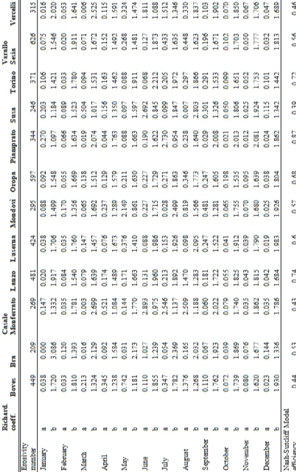
In this study the exponential relationship of Richardson coefficient (Richardson et al., 1983) in Eq. (1) above was employed to obtain the a and b parameters calibrated monthly.
The values of these coefficients for each station are reported in Table 2.
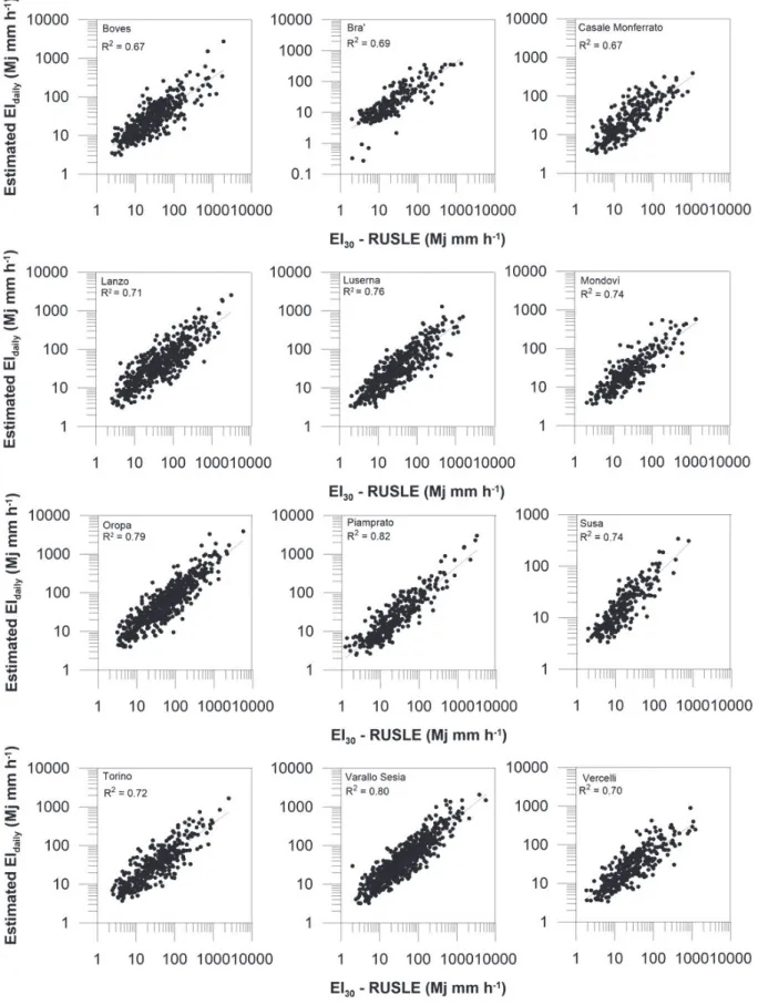
Then, this regression equation, for each station, was used to developed erosivity series starting from daily data. The erosivity data have been plotted versus the real erosivity founding a strong relationship (Fig. 2). The Nash-Sutcliffe efficiency model results (Table 2) are always higher than 0.39 showing a good performance of the twelve derived equations.
Table 2. List of monthly a and b Richardson coefficients
Fig. 2. Scatterplots between estimated (EIdaily) and measured rainfall erosivity (EI30- RUSLE) values for the calibration and fitted values.
Afterwards, starting from the daily rainfall series from 1986 to 2015, the daily erosivity equation of each month was applied to create annual, seasonal, and monthly series of rainfall erosivity.
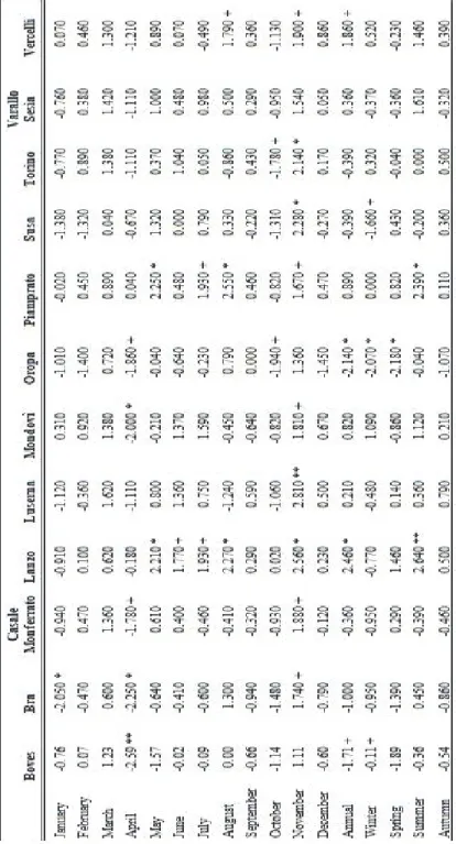
Thereafter, using the MK test, annual, seasonal, and monthly time trends during the observation period were verified, and the MK test statistics are shown in Table 3.
Table 3. Mann-Kendall trend test of rainfall erosivity using annual, seasonal, and monthly datasets of all Piedmont stations. The significance of the coefficients Z was checked for different levels of probability, p≤ ***0.001, **0.01,**0.05, and +0.10.
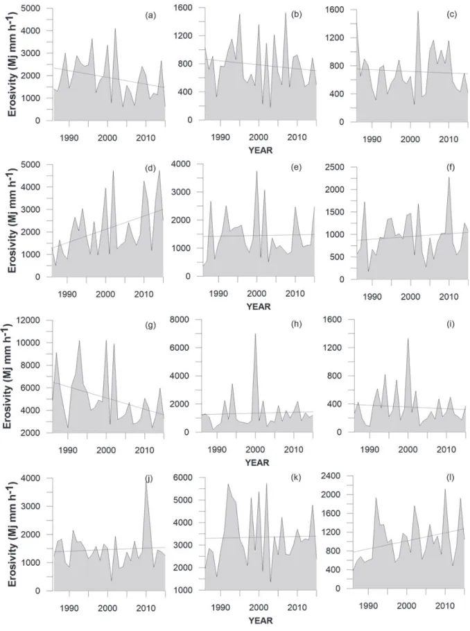
The annual rainfall erosivity experienced increasing trends in six series (Lanzo, Luserna, Mondovì, Piamprato, Varallo Sesia, and Vercelli), whereas a decreasing trend characterizes the other series (Boves, Bra, Casale Monferrato, Oropa, Susa, and Torino) (Fig. 3). Only four stations (Boves, Lanzo, Oropa, and Vercelli) show statistically significant trend in rainfall erosivity. To verify the environmental/economic impact of erosivity on agriculture, the mean annual erosivity of Piedmont has been plotted versus the wine grapes productivity from 1981 to 2015 (Fig. 4, ISTAT source). The graph shows how an increase in annual erosivity often corresponds to a clear decrease in annual wine grapes productivity. Thus, the main important economic activities of the region are strongly affected by the soil loss caused by rainfall.
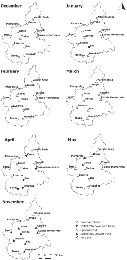
At seasonal and monthly levels, a different behaviour of rainfall erosivity emerges (Figs. 5 and 6). During winter only three stations (Mondovì, Torino, and Vercelli) show an upward statistically not significant trend. The remaining stations experienced a decrease in rainfall erosivity, which is statistically significant for Oropa and Susa. The trend signal seems to be controlled by the decrease in rainfall erosivity during the months of December and January (downward, statistically significant trend for Bra), whereas during February a general increase is recorded (Table 3). A downward trend is recorded during spring at seven stations, which is statistically significant for Boves and Oropa.
From the monthly analysis it appears, that the main responsible for the overall spring trend is April, when many stations are characterized by a downward, statistically significant trend (Boves, Bra, Casale Monferrato, Mondovì, and Oropa). During March and May, many stations show an upward trend. In summer, an increase in rainfall erosivity is detected with the exception of the stations of Boves, Casale Monferrato, and Susa (Oropa and Torino show a stationary trend). It seems that no month is mainly responsible for the summer trend. A similar trend is recorded during autumn, without any statistically significant values. The monthly analysis shows that the autumn trend is mainly influenced by the rainfall erosivity behavior during November (upward, statistically significant trend for Bra, Casale Monferrato, Lanzo, Luserna, Mondovì, Piamprato, Susa, Torino, and Vercelli).
Fig. 3. Total annual rainfall erosivity from 1986 to 2015 for (a) Boves, (b) Bra, (c) Casale Monferrato, (d) Lanzo, (e) Luserna, (f) Mondovì, (g) Oropa, (h) Piamprato, (i) Susa, (l) Torino, (m) Varallo Sesia, and (n) Vercelli.
Fig. 4. Mean annual erosivity versus annual wine grape productivity (from ISTAT) in Piedmont for the period 1981–2015.
Fig. 5. Trends in seasonal rainfall erosivity in Piedmont for the period 1986–2015.
Fig. 6. Trends in annual rainfall erosivity in Piedmont for the period 1986–2015.
5. Conclusions
In Piedmont, (Northwestrn Italy), viticulture is strongly affected by soil erosion caused by rainfall events. In this regards, the RUSLE rainfall erosion index or R- factor for twelve pluviometric stations spread in the whole region was applied to obtain a set of daily rainfall time series from a 10-minute precipitation series.
Those equations were applied to obtain the erosivity of a single erosive event from daily rainfall events greater or equal to 12.7 mm. After the application of the daily rainfall erosion index equations to the daily series of precipitation, the long- term trends of annual, monthly, and seasonal rainfall erosivity for the Piedmont region have been generated and analyzed. The main obtained results are:
− The annual rainfall erosivity experienced increasing trends in six series (Lanzo, Luserna, Mondovì, Piamprato, Varallo Sesia, and Vercelli), whereas a decreasing trend characterizes the other series (Boves, Bra, Casale Monferrato, Oropa, Susa, and Torino). Only four stations (Boves, Lanzo, Oropa and Vercelli) show statistically significant trend in rainfall erosivity.
− A widespread a decrease in rainfall erosivity, which is statistically significant for Oropa and Susa, has been recorded in winter.
− A downward trend is recorded at more than half of the stations during spring (especially in April), which is statistically significant for Boves and Oropa.
− An increase in rainfall erosivity is detected both in summer (statistically significant for Lanzo and Piamprato) and in autumn, especially during the month of November.
Acknowledgements: This work was made in the frame of the Italian MIUR Project (PRIN 2010-11)
“Response of morphoclimatic system dynamics to global changes and related geomorphological hazards”. The authors thank Arpa Piemonte for the meteorological dataset, available within a collaborative agreement between the Dipartimento di Scienze della Terra (University of Turin) and Dipartimento Sistemi Previsionali (Arpa Piemonte).
References
Acquaotta, F., Fratianni, S., 2013: Analysis on Long Precipitation Series in Piedmont (North-West Italy). Amer. J. Climate Change 2, 14–24.https://doi.org/10.4236/ajcc.2013.21002
Acquaotta, F., Fratianni, S. and Venema, V., 2016: Assessment of parallel precipitation measurements networks in Piedmont, Italy. Int. J. Climatol. 36, 3963–3974. https://doi.org/10.1002/joc.4606 Acquaotta F., Faccini F., Fratianni S., Paliaga G., Sacchini A., and Vilimek V., 2018a: Increased flash
flooding in Genoa Metropolitan Area: a combination of climate changes and soil consumption?
Meteorol. Atmos. Phys. https://doi.org/10.1007/s00703-018-0623-4
Acquaotta F., Faccini F., Fratianni S., Paliaga G., Sacchini A., 2018b: Rainfall intensity in the Genoa Metropolitan Area (Northern Mediterranean): secular variations and consequences. Weather 73, 356–363. https://doi.org/10.1002/wea.3208
Angulo-Martínez, M., and Beguería, S., 2009: Estimating rainfall erosivity from daily rainfall records: A comparison among methods using data from the Ebro Basin (NE Spain). J. Hydrol. 379, 111–121.
https://doi.org/10.1016/j.jhydrol.2009.09.051
Angulo-Martínez, M., and Beguería, S., 2012: Trends in rainfall erosivity in NE Spain at annual, seasonal and daily scales, 1955–2006. Hydrol. Earth Syst. Sci. 16, 3551–3559.
https://doi.org/10.5194/hess-16-3551-2012
Arnoldus, H.M.J., 1977: Methodology used to determine the maximum potential average annual soil loss due to sheet and rill erosion in Morocco. FAO Soil Bull. 34, 39–51.
Ateshian, J.K.H., 1974: Estimation of rainfall erosion index. J. Irrig. Drain. Div. Am. Soc. Civ. Eng.
100, 293–307.
Baronetti, A., Acquaotta F., and Fratianni, S., 2018. Rainfall variability from a dense rain gauge network in North -West Italy. Climate Res. 75, 201–213. https://doi.org/10.3354/cr01517
Bagarello, V. and D’Asaro, F., 1994: Estimating single storm erosion index. Trans. Am. Soc. Agric.
Eng. 37, 785–791. https://doi.org/10.13031/2013.28141
Borrelli, P., Diodato, N., and Panagos, P., 2016: Rainfall erosivity in Italy: a national scale spatio-temporal assessment. Int. J. Digit. Earth 9, 835 – 850. https://doi.org/10.1080/17538947.2016.1148203 Brown, L.C. and Foster, G.R., 1987: Storm erosivity using idealized intensity distribution. Trans ASAE
30, 379–386. https://doi.org/10.13031/2013.31957
Capolongo, D., Diodato, N., Mannaerts, C.M., Piccarreta, M., and Strobl, R.O., 2008: Analyzing temporal changes in climate erosivity using a simplified rainfall erosivity model in Basilicata (southern Italy). J. Hydrol. 356, 119– 130. https://doi.org/10.1016/j.jhydrol.2008.04.002
Capra, A., Porto, P., and La Spada, C., 2017: Long-term variation of rainfall erosivity in Calabria (Southern Italy). Theor. Appl. Climatol. 128, 141–158. https://doi.org/10.1007/s00704-015-1697-2 Cerro, C., Bech, J., Codina, B., and Lorente, J., 1998. Modelling rain erosivity using distrometric
techniques. Soil Sci. Soc. Amer. J. 62, 731–735.
https://doi.org/10.2136/sssaj1998.03615995006200030027x
Corti, G., Cavallo, E., Cocco, S., Biddoccu, M., Brecciaroli, G., and Agnelli, A., 2011: Evaluation of erosion intensity and some of its consequences in vineyards from two hilly environments under a Mediterranean type of climate, Italy. Soil Eros. Issues Agric. In (Eds. Godone D, Sanchi S) 01/2011, ISBN: 978-953-307-435-1.
Coutinho, M.A. and Tomas P.P., 1995: Characterisation of raindrop size distributions at the Vale Formosa experimental Erosion Center. Catena 25,187–197.
https://doi.org/10.1016/0341-8162(95)00009-H
D’Asaro, F., D’Agostino, L., and Bagarello, V., 2007: Assessing changes in rainfall erosivity in Sicily during the twentieth century. Hydrol. Proc. 21, 2862–2871. https://doi.org/10.1002/hyp.6502 Fazzini M., Fratianni S., Biancotti A., and Billi P., 2004: Skiability conditions in several skiing
complexes on Piedmontese and Dolomitic Alps. Meteorol. Zeit. 13,253–258.
https://doi.org/10.1127/0941-2948/2004/0013-0253
Ferro, V., Giordano, G., and Iovino, M., 1991: Isoerosivity and erosion risk map for Sicily. J. Hydrol.
Sci. 36, 549–564. https://doi.org/10.1080/02626669109492543
Foster, G.R., McCool, D.K., Renard, K.G., and Moldenhauer, W.C., 1981: Conversion of the Universal Soil Loss Equation to SI Metric Units. J. Soil Water Conserv. 36, 355–359.
Fratianni, S., Cassardo, C., and Cremonini, R., 2009: Climatic characterization of foehn episodes in Piedmont, Italy. Geografia Fisica e Dinamica Quaternaria 32, 15–22.
Fratianni, S., Terzago, S., Acquaotta, F., Faletto, M., Garzena, D., Prola, M.C., and Barbero, S., 2015:
How Snow and its Physical Properties Change in a Changing Climate Alpine Context?
Engineering Geology for Society and Territory - Volume 1: Clim. Change Engineer. Geol., 57-60, https://doi.org/10.1007/978-3-319-09300-0_11
Giaccone, E., Colombo N., Acquaotta, F., Paro, L., Fratianni, S., 2015: Climate variations in a high altitude Alpine basin and their effects on a glacial environment (Italian Western Alps).
Atmosfera 28, 117–128. https://doi.org/10.20937/ATM.2015.28.02.04
Hirsch, R.M., Slack, J.R., and Smith, R.A., 1982: Techniques of trend analysis for monthly water quality data. Water Resour. Res. 18, 107–121. https://doi.org/10.1029/WR018i001p00107 Hudson, N.W., 1971. Soil Conservation. Batsford Ltd, London.
Joon-Hak, L. and Jun-Haeng, H., 2011: Evaluation of estimation methods for rainfall erosivity based on annual precipitation in Korea. J. Hydrol. 409, 30–48. https://doi.org/10.1016/j.jhydrol.2011.07.031 Yu, B., Hashim, G. M., and Eusof, Z., 2001: Estimating the R-factor with limited rainfall data: A case
study from Peninsular Malaysia. J. Soil Water Conserv. 56, 101–105.
Loureiro, N.S. and Coutinho, M.A., 2001: A new procedure to estimate the RUSLE EI30 index, based on monthly rainfall data and applied to the Algarve region, Portugal. J. Hydrol. 250, 12–18.
https://doi.org/10.1016/S0022-1694(01)00387-0
Luino, F., 2005: Sequence of instability processes triggered by heavy rainfall in the northern Italy.
Geomorphology 66, 13–39. https://doi.org/10.1016/j.geomorph.2004.09.010
Nash, J.E., and Sutcliffe, J.V., 1970: River flow forecasting through conceptual models. Part I – a discussion of principles. J. Hydrol. 10, 282–290. https://doi.org/10.1016/0022-1694(70)90255-6 Petkovšek, G. and Mikoš, M., 2004: Estimating the R factor from daily rainfall data in the sub-
mediterranean climate of southwest Slovenia. Hydrol. Sci. J. 49, 869–877.
https://doi.org/10.1623/hysj.49.5.869.55134
Renard, K.G., Foster, G.R., Weesies, G.A., McCool, D.K., and Toder, D.C., 1997: Predicting soil erosion by water: a guide to conservation planning with the revised universal soil loss equation (RUSLE). USDA Agric. Handb. 703, U. S. Gov. Print Office Washington DC
Renard, K.G. and Freimund, J.R., 1994: Using monthly precipitation data to estimate the R-factor in the revised USLE. J. Hydrol. 157, 287–306. https://doi.org/10.1016/0022-1694(94)90110-4 Richardson, C.W., Foster, G.R., and Wright, D.A., 1983: Estimation of erosion index from daily
rainfall amount. Trans. ASAE 26, 153–156. https://doi.org/10.13031/2013.33893
Terzago, S., Cremonini, R., Cassardo, C, and Fratianni, S., 2012: Analysis of snow precipitation during the period 2000-09 and evaluation of a MSG/SEVIRI snow cover algorithm in SW Italian Alps. Geografia Fisica e Dinamica Quaternaria 35, 91-99.
Tropeano, D., 1984: Rate of soil erosion processes on vineyards in Central Piedmont (NW Italy).
Earth Surf. Process. Landf. 9, 253–266. https://doi.org/10.1002/esp.3290090305
Vallebona, C., Pellegrino, E., Frumento, P., and Bonari, P., 2015: Temporal trends in extreme rainfall intensity and erosivity in the Mediterranean region: a case study in southern Tuscany, Italy.
Clim. Change 128, 139–151. https://doi.org/10.1007/s10584-014-1287-9
Venema, V.K.C., Mestre, O., Aguilar, E., Auer, I., Guijarro, J.A., Domonkos, P., Vertacnik, G., Szentimrey, T., Stepanek, P., Zahradnicek, P., Viarre, J., Müller-Westermeier, G., Lakatos, M., Williams, C.N., Menne, M.J., Lindau, R., Rasol, D., Rustemeier, E., Kolokythas, K., Marinova, T., Andresen, L., Acquaotta, F., Fratianni, S., Cheval, S., Klancar, M., Brunetti, M., Gruber, C., Prohom Duran, M., Likso, T., Esteban, P., Brandsma, T., and Willett, K., 2013: AIP Conference Proceedings, 9th International Temperature Symposium on Temperature:
Its Measurement and Control in Science and Industry, ITS 2012. Vol. 1552 8, 1060–1065, https://doi.org/10.1063/1.4819690
Willmott, C.J. and Matsuura, K., 2005: Advantages of the mean absolute error (MAE) over the root mean square error (RMSE) in assessing average model performance. Clim. Res. 30, 79–82.
https://doi.org/10.3354/cr030079
Wischmeier, W.H. and Smith, D.D.,1978: Predicting rainfall erosion losses – a guide to conservation planning. USDA Sci. Educ. Adm. Agric. Res. Agric. Handb. 537, 58 pp.
Yin, S., Xie, Y., Nearing, M.A., and Wang, C., 2007: Estimation of rainfall erosivity using 5- to 60- minute fixed-interval rainfall data from China. Catena 70, 306–312.
https://doi.org/10.1016/j.catena.2006.10.011
Yu, B., Hashim, G.M., and Eusof, Z., 2001: Estimating the R-factor with limited rainfall data: a case study from peninsular Malaysia. J. Soil Water Conserv. 56, 101–105.
Yu, B., and Rosewell, C.J., 1996a: An assessment of daily rainfall erosivity model for New South Wales. Aust. J. Soil Res. 34, 139–152. https://doi.org/10.1071/SR9960139
Yu, B. and Rosewell, C.J., 1996b: A robust estimator of the R factor for the Universal Soil Loss Equation. Trans ASAE 39, 559–561. https://doi.org/10.13031/2013.27535
Yu, B. and Rosewell, C.J., 1996c: Rainfall erosivity estimation using daily rainfall amounts for South Australia. Aust. J. Soil Res. 34, 721–733. https://doi.org/10.1071/SR9960721
Zandonadi, L., Acquaotta, F., Fratianni, S., and Zavattini, J.A., 2016: Changes in precipitation extremes in Brazil (Paraná River Basin). Theor. Appl. Climatol. 123, 741–756.
https://doi.org/10.1007/s00704-015-1391-4