XXX-X-XXXX-XXXX-X/XX/$XX.00 ©20XX IEEE
Inertial sensor-based outdoor terrain classification for wheeled mobile robots
Dominik Csík
Department of Mechatronics and Automation University of Szeged
Szeged, Hungary csikd@mk.u-szeged.hu
József Sárosi
Department of Mechatronics and Automation University of Szeged
Szeged, Hungary sarosi@mk.u-szeged.hu
Ákos Odry
Department of Mechatronics and Automation University of Szeged
Szeged, Hungary odrya@mk.u-szeged.hu
Peter Sarcevic
Department of Electrical Engineering Subotica Tech
Subotica, Serbia sarcevic@vts.su.ac.rs
Abstract— Nowadays, an increasing usage of autonomous mobile robots in outdoor applications can be noticed.
Identification of the terrain type is very important for efficient navigation. In this paper, a novel method is proposed for terrain classification in the case of wheeled mobile robots. The classification algorithm uses frequency domain features, which are extracted in fixed-size windows, and Multi-Layer Perceptron (MLP) neural networks as classifiers. Data from inertial sensors were collected for different outdoor terrain types using a prototype measurement system. The data of the accelerometer and the gyroscope were tested separately and together, and different processing window sizes were also applied. The achieved results show that above 99% classification efficiency can be achieved using the collected data.
Keywords— mobile robots, inertial sensors, frequency domain analysis, feature extraction, pattern recognition
I. INTRODUCTION
Autonomous mobile robots are used in a large variety of outdoor field applications, such as agriculture, environmental monitoring, military applications, etc. Knowledge of the environment, such as the terrain type, can be used as important information for efficient navigation [1, 2].
Terrain classification for wheeled mobile robots is usually performed using cameras [3, 4], lasers [3], and inertial sensors [2, 5-9], but sound-based recognition was also reported in related works [10]. The fusion of different sensor types can be also applied [2, 3]. Some approaches using walking robots for classifying terrains also exist [11].
The most used inertial sensors in the case of mobile robots are the accelerometer and the gyroscope. Accelerometers measure linear acceleration along one or more axes, while gyroscopes measure angular velocity around one or more axes. These sensors can be applied for control [12-14], position and orientation estimation [15-16], etc.
In related works, which apply inertial sensors for terrain classification, mostly only vibrations recorded by accelerometers were applied [2, 6-8]. The use of gyroscopes together with accelerometers was also reported in the literature [9].
In [2], only the Z-axis of the accelerometer was utilized to classify 5 pavement types. The Root Mean Square (RMS) feature was used during classification, and the results showed above 80% accuracy.
The authors of [6] proposed a Recurrent Neural Network (RNN)-based method, which did not apply any feature computation on the signals of the three-axis sensor. An average accuracy of roughly 85% was achieved for the dataset consisting of 14 terrain types.
Vicente et al. extracted altogether 523 features using Power Spectrum Density (PSD)-based and 11 different statistical features to classify 4 indoor surface types [7]. The size of the feature vector was reduced using the Principal Component Analysis (PCA) algorithm.
In [8], different time domain and frequency domain features were extracted from the signals of the Z-axis, which were recorded with 100 Hz. A Laplacian Support Vector Machine (LapSVM) was used to classify 6 outdoor terrain types.
The authors of [9] applied more than 800 features extracted from measurements recorded using an accelerometer and a gyroscope. The Linear Bayes Normal Classifier was applied to classify indoor terrain types into 4 classes.In this study, frequency domain-based features extracted from inertial sensor signals are applied for the classification of outdoor terrain types. Based on related works, it was reasonable to test the applicability of the inertial sensor types in this application. The effect of the processing window size is also tested, since it can affect the reaction time during transitions between different terrain types.
II. EXPERIMENTAL SETUP A. Measurement System
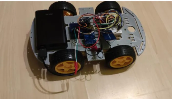
A wheeled mobile robot, which can be seen in Fig. 1, was constructed for collecting measurement data. The robot has four wheels, of which two are driven. The size of the mobile robot is 158 x 255 x 45 mm, the distance between the wheels is 132 mm in width and 116 mm is length, and the mass of the mobile robot is 595 g.
An ESP32 board is used for motor control through an L9110 controller, communication with the sensors and storage of the measurement data. Measurement data are stored on an SD card.
The robot is equipped with a 9 degrees of freedom (9DoF) inertial sensor board, which is made up of an ADXL345 tri- axial MicroElectroMechanical System (MEMS) accelerometer, an ITG3200 tri-axial MEMS gyroscope, and D. Csík, Á. Odry, J. Sárosi and P. Sarcevic: Inertial sensor-based outdoor terrain classification for wheeled mobile robots, IEEE International Symposium on Intelligent Systems and Informatics (SISY), Subotica, Serbia, pp. 159-164 (2021). DOI: 10.1109/SISY52375.2021.9582504
© 2021 IEEE
an HMC5883L tri-axial magnetometer. The ADXL345 can measure up to ± 16 g in 13-bit resolution with the highest sampling rate of 3.2 kHz, while the gyroscope features a 16- bit analog-to-digital converter, and it can measure angular rate in a range of ± 2000 deg/s with 8 kHz frequency. In this study, only the accelerometer and the gyroscope are utilized.
B. Data Acquisition
The prototype measurement system was used to collect data, which can be used later to construct the classifier.
Data acquisition was done on 6 different outdoor terrains, which can be seen if Fig. 2, and are the following:
1. Concrete 2. Grass 3. Pebbles 4. Sand 5. Paving stone
6. Synthetic running track
The applied sampling frequency for both sensors was 500 Hz. One measurement session was 4.5 s long and data for all six classes were recorded in 7 sessions, which means 31.5 s for all terrain types.
III. CLASSIFICATION ALGORITHM
The proposed classification algorithm, which can be seen in Fig. 3, consists of four stages. In the first stage, error compensation is performed on the measurements. Windowing is performed in the second stage, while feature extraction on the data in the processing window is performed in the third stage. In the fourth stage, the classifier determines the terrain type using the extracted features.
A. Error Compensation
The deterministic errors are compensated in this phase using calibration parameters obtained utilizing an evolutionary algorithm-based method [17]. The algorithm applies measurements recorded in different stationary orientations to compute the required parameters.
B. Windowing
Windowing is performed using fixed window sizes and constant shift sizes. Multiple processing window sizes were tested to explore its effect on the recognition efficiency, which are 128, 256, and 512 samples, which means nearly 0.25 s, 0.5 s, and 1 s in the case of the applied 500 Hz sampling frequency. To construct more training and validation data, the utilized shift size was 32 samples.
C. Feature Extraction
Features are extracted using the measurements in the processing window. The algorithm uses only frequency domain features, which can possibly carry important information of the terrain type. The transformation from time domain to frequency domain was done using the Fast Fourier Transform (FFT) algorithm. The selected features are the following [18]:
• Spectral energy (ENE) – The spectral energy can be computed as:
ENE = ∑𝑀 𝑌𝑖2
𝑖=1 ()
where M is the number of points in the frequency axis, and Yi is the value of the amplitude spectrum at the given frequency index.
• Median frequency (MDF) – The frequency which divides the spectrum into two regions with equal amplitude.
∑MDF𝑖=1 𝑌𝑖= ∑𝑀𝑖=MDF𝑌𝑖=1
2∑𝑀𝑖=1𝑌𝑖 () Fig. 1. Wheeled mobile robot used for data acquisition.
Fig. 2. Tested outdoor terrain types: a) concrete; b) grass; c) pebbles; d) sand; e) paving stone; f) synthetic running track.
Fig. 3. Parts of the classification algorithm.
• Mean frequency (MNF) – This frequency is also called central frequency (fc), and it can be calculated using the following equation.
MNF = ∑𝑀 𝑓𝑖𝑌𝑖 𝑖=1 ∑𝑀 𝑌𝑖
⁄ 𝑖=1 () where fi is the frequency at the given index.
• Mean power (MNP) – The average power of the spectrum (4).
MNP = ∑𝑀 𝑌𝑖
𝑖=1 ⁄𝑀 ()
• Peak magnitude (PKM) – The highest amplitude in the spectrum.
• Peak frequency (PKF) – The frequency at which the PKM occurs.
• Variance of the central frequency (VCF) – The variance of the central frequency can be defined using (5).
VCF = 1
∑𝑀𝑖=1𝑌𝑖∑𝑀𝑖=1𝑌𝑖(𝑓𝑖− 𝑓𝑐)2 () D. Classifier
Various classification methods can be applied in such pattern recognition applications. E.g., SVMs [8], fuzzy rule- based classifiers [19], the k-Nearest Neighbour (k-NN) method [20], decision trees or Classification Trees (CT) [20], Multi-Layer Perceptron (MLP) neural networks [20], the Naïve Bayes Classifier (NBC) [20], etc.
MLP classifiers were applied in this research, which are feedforward Artificial Neural Networks (ANNs). These classifiers proved to be very applicable for online classification tasks [20]. In MLPs, neurons are organized into three or more layers, an input, an output, and one or more hidden layers. Each layer is fully connected to the next one using weighted connections. A neuron has an activation function that maps the sum of its weighted inputs to the output.
These ANNs are usually trained using the backpropagation algorithm.
The input of the MLP is composed of the computed features, and a neuron is assigned to each class in the output layer. To make the network easily implementable on the used hardware, only one hidden layer is utilized, which is tested with different number of neurons in the layer, to find the optimal configuration. The hyperbolic tangent sigmoid transfer function was used in the hidden layer, while the linear activation function was applied in the output layer.
IV. EXPERIMENTAL RESULTS A. Classification
Measurements from 4 of the 7 sessions were used as training datasets, and the remaining 3 sessions for the validation of the trained classifiers with unknown data.
All 7 selected feature types were extracted for signals of all three sensor axes, so, altogether 21 features were computed for each sensor type.
The training of the MLP neural networks was tested using 1-15 hidden layer neurons. The 70% of the training data were used as training inputs, and the remaining 30% as validation inputs for the training method.
The highest output at the neurons of the output layer was determined as the class of the current terrain type.
Classification efficiency was calculated using the following equation:
𝐸(%) =𝑁𝑐
𝑁𝑠∙ 100, () where E is the recognition rate in percentages, Nc is the number of correctly classified samples, and Ns is the number of all samples in the dataset.
To explore the capability of the two sensor types in this application, they were tested separately and together in the case of all processing window sizes. In later comparison, for each setup, the results with highest recognition efficiency on validation data were chosen, which are the sessions which were not used during the training of the MLPs.
B. Performance Evaluation
The obtained classification efficiencies on training and validation datasets per used sensor types can be seen in Table I and Table II, respectively.
A convergence in recognition rate was noticed for all setups in the case of required hidden layer neurons, which means that the tested numbers are sufficient.
The achieved classification efficiencies show a rising tendency by increasing the size of the processing window. In the case of training datasets, above 99% can be achieved using both sensors, even when the smallest window size is applied.
The effect of the window size is bigger when only one sensor is used. Between the smallest and the biggest window size an increase of around 3.5% can be noticed in the case of the gyroscope, while in the case of the accelerometer, the efficiency increases by more than 6.5%. A stronger effect can be noticed at unknown data. The difference between the recognition rates is 5.08% and 13.87% for the gyroscope and the accelerometer, respectively. The increase is smaller, around 2.5%, when the two sensors are used together.
If only one sensor is utilized, it can be noticed that the gyroscope provides higher efficiencies than the accelerometer. In the case of training data, the difference is 3.17% for the smallest window, 2.45% for the medium sized window, and 0.08% for the largest applied window. In the case of validation data, the differences are much more significant, 17.58%, 14.55%, and 8.79% for the small, medium, and large windows, respectively. It can be also stated based on the results, that the fusion of the two sensor types provides the highest recognition rates. Using both sensors, compared to the results obtained with the gyroscope data, the increase is below 3% in the case of training data, because, even with the smallest window, above 96% classification efficiency can be achieved using the gyroscope. The difference is bigger in the case of unknown data, especially for the smallest window size, where the difference is 4.48%. The difference is below 2% in the case of the two larger windows.
The highest achieved recognition rate on validation data was 99.70%, which was obtained by fusing the data of the two sensors and applying the largest window. Using only one sensor, the gyroscope provided 97.78% using the largest processing window. In the case of the smallest window, 97.18% can be achieved by using the data of the two sensors together, and 92.70% with the gyroscope. The accelerometer, which is the most widely used sensor type in this application,
provided only 88.99% and 75.12% with the largest and smallest window, respectively.
The gyroscope and the two sensors together provide above 90% efficiencies on unknown samples, thus, the number of misclassifications is small. In the case of the accelerometer, it is important to investigate between which classes do the misclassifications occur and where does the increasing of the processing window size help. Table III shows the recognition rates per class on validation data in the case when only data from the accelerometer were utilized with the smallest and the largest processing windows. The overall recognition rates were 75.12% and 88.99%, respectively. Table IV and Table V show the confusion matrices for the same setups. The corresponding terrain types to class numbers are the same as given in section II.B. It can be seen from Table III, that grass was recognized in both setups with 100% efficiency, while only 2.49% and 4.91% improvement was obtained by increasing the processing window size in the case of pebbles and synthetic running track, respectively. Significant improvement, almost 20%, can be noticed for concrete and sand, while nearly 30% was obtained in the case of paving stones. The confusion matrices show that above 20%
misclassification rate occurs between concrete and paving stone, which almost totally disappears by increasing the window width. In the case of pebbles, which is the class with the lowest recognition rates, 64.18% and 66.67%, 33.33% of the samples were classified as grass with the smallest window, while by increasing the window size this rate decreased to 0%
and a 33.33% misclassification rate appeared at class 6, which was 0.5% with the smallest processing window size.
TABLE I. CLASSIFICATION EFFICIENCIES ON TRAINING DATASETS
Window width
Sensor
gyroscope accelerometer gyroscope + accelerometer
128 96.33% 93.16% 99.13%
256 98.68% 96.23% 100%
512 99.85% 99.77% 100%
TABLE II. CLASSIFICATION EFFICIENCIES ON VALIDATION DATASETS
Window width
Sensor
gyroscope accelerometer gyroscope + accelerometer
128 92.70% 75.12% 97.18%
256 97.09% 82.54% 98.68%
512 97.78% 88.99% 99.70%
TABLE III. RECOGNITION RATES PER CLASS (%) ON VALIDATION DATA WHEN ONLY ACCELEROMETER MEASUREMENTS WERE USED WITH THE
SMALLEST AND THE LARGEST PROCESSING WINDOWS
Window width
Class
1 2 3 4 5 6
128 70.64 100.00 64.18 69.10 63.18 83.57 512 98.79 100.00 66.67 87.88 92.12 88.48
TABLE IV. CONFUSION MATRIX (%) ON VALIDATION DATA WHEN ONLY ACCELEROMETER MEASUREMENTS WERE USED WITH THE SMALLEST
PROCESSING WINDOW
Target class
1 2 3 4 5 6
Output class
1 0.50 9.00 22.39 0.50
2 33.33 2.49
3 1.00
4 8.46 1.49 13.43 14.93
5 20.90 16.92
6 0.50 2.49 1.00
TABLE V. CONFUSION MATRIX (%) ON VALIDATION DATA WHEN ONLY ACCELEROMETER MEASUREMENTS WERE USED WITH THE LARGEST
PROCESSING WINDOW
Target class
1 2 3 4 5 6
Output class
1 5.45 3.03
2 3
4 1.21 4.85 11.52
5 6.67
6 33.33
V. CONCLUSION
In this paper, a novel method was proposed for the classification of different terrain types for wheeled mobile robots. The classification algorithm applies spectral features and MLP neural networks. The inertial sensors were tested separately and together, and different processing window sizes were also tested.
The results show that significantly higher recognition rates can be achieved using the signals of the gyroscope sensor than with using only the accelerometer. The classification efficiencies increase by fusing the two sensor types.
The classification efficiencies show a rising tendency by increasing the processing window size, but even with the smallest tested window size, 92.70% can be achieved on validation data utilizing only the gyroscope, and 97.18%
applying both sensors. The highest classification efficiencies on unknown data were obtained using the largest window size, which were 97.78% and 99.70% with the gyroscope and the fused data, respectively.
Future goals include the expansion of the algorithm with different indoor terrain types, the testing of the effect of different speeds on the algorithm, and finding the features with the highest effect.
REFERENCES
[1] A. Dutta and P. Dasgupta, “Ensemble learning with weak classifiers for fast and reliable unknown terrain classification using mobile robots,”
IEEE Trans. Syst. Man Cybern. Syst., vol. 47, pp. 2933-2944, November 2016.
[2] F. Oliveira, E. Santos, A. A. Neto, M. Campos, and D. Macharet,
“Speed-invariant terrain roughness classification and control based on inertial sensors,” in Proc. of Latin American Robotics Symposium (LARS) and Brazilian Symposium on Robotics (SBR), 2017, pp. 1-6.
[3] M. Häselich, M. Arends, N. Wojkeb, F. Neuhausa, and D. Paulus,
“Probabilistic terrain classification in unstructured environments,”
Robot. Auton. Syst., vol. 61, pp. 1051-1059, 2013.
[4] Y. N. Khan, P. Komma, K. Bohlmann, and A. Zell, “Grid-based visual terrain classification for outdoor robots using local features,” in Proc.
of IEEE Symposium on Computational Intelligence in Vehicles and Transportation Systems (CIVTS), 2011, pp. 16-22.
[5] M. Mei, J. Chang, Y. Li, Z. Li, X. Li, and W. Lv, “Comparative study of different methods in vibration-based terrain classification for wheeled robots with shock absorbers,” Sensors, vol. 19, 1137, March 2019.
[6] S. Otte, C. Weiss, T. Scherer, and A. Zell, “Recurrent neural networks for fast and robust vibration-based ground classification on mobile robots,” in Proc. of IEEE International Conference on Robotics and Automation (ICRA), 2016, pp. 1-6.
[7] A. Vicente, J. Liu, and G.-Z. Yang, “Surface classification based on vibration on omni-wheel mobile base,” in Proc. of IEEE/RSJ International Conference on Intelligent Robots and Systems (IROS), 2015, pp. 916-921.
[8] W. Shi, Z. Li, W. Lv, Y. Wu, J. Chang, and X. Li, “Laplacian support vector machine for vibration-based robotic terrain classification,”
Electronics , vol. 9, 513, March 2020.
[9] D. Tick, T. Rahman, C. Busso, and N. Gans, “Indoor robotic terrain classification via angular velocity based hierarchical classifier selection,” in Proc. of IEEE International Conference on Robotics and Automation (ICRA), 2012, pp. 3594-3600.
[10] A. Valada, L. Spinello, and W. Burgard, “Deep Feature Learning for Acoustics-Based Terrain Classification,” in Springer Proceedings in Advanced Robotics: Robotics Research, 2017, pp. 21-37.
[11] K. Walas, “Terrain classification and negotiation with a walking robot,” J Intell Robot Syst, vol. 78, pp. 401-423, 2015.
[12] Á. Odry, J. Fodor, and P. Odry, “Stabilization of a two-wheeled mobile pendulum system using LQG and fuzzy control techniques,”
International Journal On Advances in Intelligent Systems, vol. 9, pp.
223-232, January 2016.
[13] A. Papp, L. Szilassy, and J. Sarosi, “Navigation of differential drive mobile robot on predefined, software designed path,” Recent Innovations in Mechatronics, vol. 3, pp. 1-5, September 2016.
[14] J. Simon, “Autonomous wheeled mobile robot control,”
Interdisciplinary Description of Complex Systems: INDECS, vol. 15, pp. 222-227, 2017.
[15] Á. Odry, I. Kecskes, P. Sarcevic, Z. Vizvari, A. Toth, and P. Odry, “A novel fuzzy-adaptive extended kalman filter for real-time attitude estimation of mobile robots,” Sensors, vol. 20, 803, 2020.
[16] J. Simon and G. Martinovic, “Navigation of mobile robots using wsn’s rssi parameter and potential field method,” Acta Polytech. Hung., vol.
10, pp. 107-118, 2013.
[17] P. Sarcevic, Sz. Pletl, and Z. Kincses, “Evolutionary algorithm based 9dof sensor board calibration,” in Proc. of IEEE International Symposium on Intelligent Systems and Informatics (SISY), 2014, pp.
187-192.
[18] P. Sarcevic, Sz. Pletl, and Z. Kincses, “Comparison of time- and frequency-domain features for movement classification using data from wrist-worn sensors,” in Proc. of IEEE International Symposium on Intelligent Systems and Informatics (SISY), 2017, pp. 261-266.
[19] A. Tormasi and L. T. Koczy, “Rule-base parameter optimization for a multi-stroke fuzzy-based character recognizer,” in Advances in Intelligent Systems Research: Proc. of the 2015 Conference of the International Fuzzy Systems Association and the European Society for Fuzzy Logic and Technology (IFSA-EUSFLAT), 2015, pp. 1331-1337.
[20] P. Sarcevic, Z. Kincses, and Sz. Pletl, “Online human movement classification using wrist-worn wireless sensors,” J. Amb. Intel. Hum.
Comp., vol. 10, pp. 89-106, January 2019.