CERS-IE WORKING PAPERS | KRTK-KTI MŰHELYTANULMÁNYOK
INSTITUTE OF ECONOMICS, CENTRE FOR ECONOMIC AND REGIONAL STUDIES, BUDAPEST, 2020
Regional differences in diabetes across Europe – regression and causal forest analyses
PÉTER ELEK – ANIKÓ BÍRÓ
CERS-IE WP – 2020/27
June 2020
https://www.mtakti.hu/wp-content/uploads/2020/06/CERSIEWP202027.pdf
CERS-IE Working Papers are circulated to promote discussion and provoque comments, they have not been peer-reviewed.
Any references to discussion papers should clearly state that the paper is preliminary.
Materials published in this series may be subject to further publication.
ABSTRACT
We examine regional differences in diabetes within Europe, and relate them to variations in socio-economic conditions, comorbidities, health behaviour and diabetes management. Using SHARE (Survey of Health, Ageing and Retirement in Europe) data, first, we estimate multivariate regressions, where the outcome variables are diabetes prevalence, diabetes incidence, and weight loss due to diet as an indicator of management. Second, we study the heterogeneous impact of the risk factors on the regional differences in incidence with causal random forests.
Compared to Western Europe, the transition odds to diabetes is 2.3-fold in Southern and 2.7-fold in Eastern Europe, which decreases to 2.0 and 2.1 after adjusting for individual characteristics. The remaining differences are explained by country-specific healthcare indicators. Based on the causal forest approach, the adjusted East-West difference is essentially zero for the lowest risk groups (tertiary education, no hypertension, no overweight) and increases substantially with these risk factors, but the South-West difference is much less heterogeneous. The prevalence of diet-related weight loss around the time of diagnosis also exhibits regional variation. The results suggest that more emphasis should be put on diabetes prevention among high-risk individuals in Eastern Europe.
JEL codes: C21, C45, I10, I12, I14
Keywords: causal forest, diabetes, Europe, health behaviour, SHARE data
Péter Elek
Department of Economics, Eötvös Loránd University, 1112 Budapest, Pázmány Péter sétány 1/a
and
Health and Population Lendület Research Group, Centre for Economic and Regional Studies, 1097 Budapest, Tóth Kálmán u. 4.
e-mail: peter.elek@tatk.elte.hu
Anikó Bíró
Health and Population Lendület Research Group, Centre for Economic and Regional Studies, 1097 Budapest, Tóth Kálmán u. 4.
e-mail: biro.aniko@krtk.mta.hu
A cukorbetegség regionális különbségei Európában – regressziós és oksági erdő alapú elemzések
ELEK PÉTER – BÍRÓ ANIKÓ
ÖSSZEFOGLALÓ
A cukorbetegség regionális különbségeit vizsgáljuk Európában, és ezeket összefüggésbe hozzuk a szocioökonómiai tényezők, társbetegségek, egészségmagatartás és diabétesz-menedzsment eltéréseivel. A SHARE (Survey of Health, Ageing and Retirement in Europe) adatfelvételt használva először többváltozós regressziókkal becsüljük a cukorbetegség prevalenciájára és incidenciájára, valamint az étrendi alapú testsúlycsökkenés előfordulására – mint a kezelés egy indikátorára – ható tényezőket. Másodszor, oksági erdők (causal forests) segítségével elemezzük a kockázati tényezők heterogén hatását az incidencia regionális eltéréseire.
Nyugat-Európához képest a cukorbeteggé válás esélye (odds) 2,3-szeres Dél- Európában és 2,7-szeres Kelet-Közép-Európában. Az esélyhányadosok 2,0-re és 2,1-re csökkennek az egyéni tényezőkre való kontrollálás után, és a fennmaradó különbségeket teljesen magyarázzák az országspecifikus egészségügyi indikátorok különbségei. Az oksági erdő alapú becslések szerint az incidencia egyéni tényezőkre kontrollált Kelet-Nyugat közötti eltérése lényegében zérus a legkisebb kockázatú csoportokban (felsőfokú végzettség, nincs magas vérnyomás, nincs túlsúly), és jelentősen növekszik ezekkel a kockázati tényezőkkel, míg a Dél vs. Nyugat eltérés sokkal kevésbé változékony a kockázati tényezők szerint. Az étrendi alapú testsúlycsökkenés prevalenciája is mutat regionális különbségeket. Eredményeink szerint Kelet-Közép-Európában a korábbiaknál nagyobb hangsúlyt kell helyezni a cukorbetegség megelőzésére a magas kockázatú csoportokban.
JEL: C21, C45, I10, I12, I14
Kulcsszavak: cukorbetegség, egészségmagatartás, Európa, oksági erdő, SHARE adatok
Regional differences in diabetes across Europe – regression and causal forest analyses
P´ eter Elek
*1,2and Anik´ o B´ır´ o
11Health and Population “Lend¨ulet” Research Group, Centre for Economic and Regional Studies, Budapest, Hungary
2Department of Economics, E¨otv¨os Lor´and University (ELTE), Budapest, Hungary
June 15, 2020
Abstract
We examine regional differences in diabetes within Europe, and relate them to variations in socio-economic conditions, comorbidities, health behaviour and diabetes management. Using SHARE (Survey of Health, Ageing and Retirement in Europe) data, first, we estimate multivariate regressions, where the outcome variables are di- abetes prevalence, diabetes incidence, and weight loss due to diet as an indicator of management. Second, we study the heterogeneous impact of the risk factors on the regional differences in incidence with causal random forests.
*E-mail: peter.elek@tatk.elte.hu
E-mail: biro.aniko@krtk.mta.hu
Compared to Western Europe, the transition odds to diabetes is 2.3-fold in South- ern and 2.7-fold in Eastern Europe, which decreases to 2.0 and 2.1 after adjusting for individual characteristics. The remaining differences are explained by country-specific healthcare indicators. Based on the causal forest approach, the adjusted East-West dif- ference is essentially zero for the lowest risk groups (tertiary education, no hypertension, no overweight) and increases substantially with these risk factors, but the South-West difference is much less heterogeneous. The prevalence of diet-related weight loss around the time of diagnosis also exhibits regional variation. The results suggest that more emphasis should be put on diabetes prevention among high-risk individuals in Eastern Europe.
Keywords: causal forest, diabetes, Europe, health behaviour, SHARE data JEL codes: C21, C45, I10, I12, I14
Acknowledgments: The authors were supported by the “Lend¨ulet” programme of the Hungarian Academy of Sciences (grant number: LP2018-2/2018). P´eter Elek was supported by the J´anos Bolyai Research Scholarship of the Hungarian Academy of Sciences and by the by the ´UNKP-19-4 New National Excellence Programme of the Hungarian Ministry for Innovation and Technology. The authors would like to thank No´emi Kreif and participants at the annual conference of the Hungarian Society of Economists as well as at the annual conference of the Austrian Health Economics Association for useful comments.
1 Introduction
Living with diabetes mellitus is associated with increased all-cause mortality as well as mor- tality due to cardiovascular disease, chronic lower respiratory diseases, influenza, pneumonia, and kidney disease [Li et al., 2019]. More recently, diabetes has been shown to increase the mortality rate and the progression to severe disease in COVID-19 around twofold [Huang et al., 2020].
In this paper, our aim is to document regional differences in the prevalence and incidence of diabetes across Europe, and to relate these differences to variations in socio-economic conditions, comorbidities, health behaviour and diabetes management. Around 8.9% of Europeans aged 20-79 years live with diabetes, and 8.5% of all deaths is attributable to diabetes and its complications [IDF, 2019]. However, the regional distribution is very uneven:
prevalence shows a more than twofold and mortality a more than fourfold difference even across the member states of the European Union (Whiting et al., 2011, IDF, 2019). It is well known that genetics, lifestyle, diet and the healthcare system all influence the incidence and mortality in diabetes, and these risk factors are unevenly distributed across the population of European countries [Tamayo et al., 2014]. In particular, the roles of socio-economic inequalities (Agardh et al., 2011, Espelt et al., 2013), of the body mass index (e.g. Narayan et al., 2007) and of lifestyle changes (e.g. Knowler et al., 2002) are well documented.
However, less is known about the relative role of the above factors in explaining the variation of diabetes across Europe. To examine this question, we make use of waves 4−7 of the Survey of Health, Ageing and Retirement in Europe (SHARE) [B¨orsch-Supan, 2019].1
1This paper uses data from SHARE Waves 1, 2, 3, 4, 5, 6 and 7 (DOIs: 10.6103/SHARE.w1.700, 10.6103/SHARE.w2.700, 10.6103/SHARE.w3.700, 10.6103/SHARE.w4.700, 10.6103/SHARE.w5.700, 10.6103/SHARE.w6.700, 10.6103/SHARE.w7.700), see B¨orsch-Supan et al. [2013] for methodological
SHARE is a cross-national panel database of micro data on demographic, socio-economic, labour market, health and lifestyle information of about 140,000 individuals in Europe aged 50 or older, hence it is a convenient database for analysing all important diabetes-related factors simultaneously. Indeed, a number of studies have used SHARE for diabetes re- search, e.g. to analyse the relationship of diabetes with hospital admissions and mortality [Rodriguez-Sanchez and Cantarero-Prieto, 2019], with socio-economic status [Espelt et al., 2013], with labour force exit (Rumball-Smith et al., 2014, Kouwenhoven-Pasmooij et al., 2016) and with depression [Bashkin et al., 2018]. We contribute to the existing literature by analysing transition to diabetes on a six-year horizon (not just the prevalence) with a focus on differences between the three regions of Europe, by the application of causal forests to analyse heterogeneous differences, and by relating the transition patterns to weight loss as an indicator of diabetes management.
The risk factors for diabetes are highly correlated and may influence diabetes prevalence and incidence in a nonlinear and non-additive way. For instance, the combination of obesity, hypertension, slightly elevated blood sugar and abnormal cholesterol level markedly increases the risk of cardiovascular disease and the transition rate to overt diabetes. This is the rationale behind the diagnosis of the metabolic syndrome, which is defined, roughly, when a patient has at least three risk factors out of the above four. Some studies argue that metabolic syndrome is more than its parts in terms of cardiovascular or overt diabetes risk (but see
details. The SHARE data collection has been primarily funded by the European Commission through FP5 (QLK6-CT-2001-00360), FP6 (SHARE-I3: RII-CT-2006-062193, COMPARE: CIT5-CT-2005-028857, SHARELIFE: CIT4-CT-2006-028812) and FP7 (SHARE-PREP: No211909, SHARE-LEAP: No227822, SHARE M4: No261982). Additional funding from the German Ministry of Education and Research, the Max Planck Society for the Advancement of Science, the U.S. National Institute on Aging (U01 AG09740- 13S2, P01 AG005842, P01 AG08291, P30 AG12815, R21 AG025169, Y1-AG-4553-01, IAG BSR06-11, OGHA 04-064, HHSN271201300071C) and from various national funding sources is gratefully acknowledged (seewww.share-project.org).
e.g. Kassi et al., 2011 for a review of controversies), suggesting interaction effects between the risk factors. We train a causal random forest developed by Wager and Athey [2018] and Athey et al. [2019] to investigate heterogeneity in the adjusted regional differences in diabetes incidence. Finally, we investigate regional differences in the change in health behaviour (the probability of weight loss due to diet) around the time of diabetes diagnosis. The results shed light on the origins of the marked cross-country differences in diabetes throughout Europe.
2 Data
The SHARE surveys were conducted in seven waves, starting in 2004, and the currently last wave was taken in 2017. The number of participating countries gradually expanded from 12 to 27 to include new EU member states as well. We exploit the panel nature of the survey by using waves 4 and 7, which were taken six years apart (2011 and 2017), hence transition to diabetes can be reliably examined on them. We split the 15 countries that appear in both waves into three groups: West [including North] (Austria, Belgium, Denmark, France, Germany, Sweden, Switzerland); South (Italy, Portugal, Spain); East (Czech Republic, Estonia, Hungary, Poland, Slovenia).2 We use calibrated weights to avoid bias due to unit nonresponse and panel attrition (see Malter and B¨orsch-Supan, 2015 for details).
In our analysis, we treat a person as having diabetes if he / she answered “yes” to any of the following two questions: (1) “Has a doctor ever told you that you had / Do you currently
2We use data from waves 4 and 7 to ensure that at least three countries are present from each region and a sufficient number of transitions to diabetes is observed. Hungary, Poland and Portugal were not included in wave 5, Hungary did not appear in wave 6, either.
have diabetes or high blood sugar?” (2) “Do you currently take drugs at least once a week for diabetes or high blood sugar?” We examine diabetes prevalence, i.e. the binary indicator of having diabetes in wave 7; and diabetes incidence (transition to diabetes), i.e. the binary indicator of having diabetes in wave 7 among those who did not have diabetes in wave 4. We do not distinguish between Type 1 and Type 2 diabetes, but around 90% of the prevalence and the overwhelming majority of incidence above 50 years belongs to the latter category [IDF, 2019].
Other variables – which we use as explanatory variables – include region, demographic and socio-economic characteristics (gender, age, years of education), body mass index (BMI, calculated from self-reported height and weight, and then categorised into normal weight (BM I < 25), overweight (25 ≤ BM I < 30), obesity (30 ≤ BM I) and, as a subgroup, severe obesity (35 ≤ BM I)), comorbidities (hypertension and high cholesterol, measured by drug use on these conditions) and lifestyle factors (binary indicators of smoking now;
playing sports at least once a week; eating fruits or vegetables daily). Since the lifestyle variables were not recorded for all respondents in wave 7, we can use them only from wave 4. The dataset also contains the self-reported binary indicator of having lost weight due to diet during the past 12 months in wave 7.
We merge three country-specific healthcare indicators to the SHARE data: total health- care spending per GDP (source: Eurostat, 2020); the number of physicians per 1,000 inhab- itants (source: WHO, 2020); and the share of the population aged 16 and above who report unmet needs for medical care due to financial reasons, waiting lists or having to travel too far (source: Eurostat, 2020). The indicators refer to year 2011 (the time of wave 4), except for health spending per GDP, which refers to year 2013 (due to missing data in 2011).
3 Methods
3.1 Multivariate regressions
We fit linear probability and logit models on diabetes prevalence and incidence, respec- tively. We include gradually more control variables beyond the regional dummies (or in some specifications the country dummies) to examine their confounding effect on regional / cross-country differences. First, we add the socio-economic indicators (age, age squared, gender and education categories). Then, we extend the models with indicators of health sta- tus (BMI categories, hypertension, high blood cholesterol) and health behaviour (smoking, weekly sports activity and daily fruit or vegetable consumption).3 As the last extension, we add the country-specific healthcare indicators to the explanatory variables to check whether they explain the remaining part of regional differences.
We also investigate the change in health behaviour around the time of diabetes diagnosis.
Specifically, we estimate linear and logit models of the probability of weight loss due to diet in wave 7. We fit these models on the sample of individuals who were not diabetic in wave 4, and use the interaction of the regional dummies with the wave 7 diabetes dummy (and other controls) to investigate regional heterogeneities in the change of the prevalence of weight loss due to the diagnosis of diabetes.
3We experimented with the addition of a rich set of further controls such as household size, marital status, labour market status, childhood health or alcohol consumption. These controls turned out to be statistically insignificant and their inclusion in the models did not change the coefficients of the regional dummies.
3.2 Causal forests
In order to analyse the heterogeneous effect of the risk factors on the regional differences in diabetes incidence, we train causal forests separately on East-West and South-West differ- ences (in each analysis we omit the third category from the sample). Specifically, let Wi be the regional dummy (which takes one for East or South and zero for West) and Xi denote the control variables. Let Yi(1) = Yi(Wi = 1) and Yi(0) = Yi(Wi = 0) be the potential outcomes, i.e. the diabetes status of a particular person in the (imagined) situation that she is in Eastern (Southern) or in Western Europe, respectively. We seek to estimate the conditional “treatment” effect
τ(x) =E(Yi(1)−Yi(0)|Xi =x)
assuming unconfoundedness and overlap.4 The unconfoundedness assumption states that {Yi(1), Yi(0)}are independent from Wi conditional on the value ofXi,while overlap means that 0< p(x)<1, where p(x) = Pr (Wi = 1|Xi =x) is the propensity score.
The fundamental problem of estimating treatment effects lies in the fact that for each i we only observe either Yi(1) or Yi(0), not both. Still, unconfoundedness ensures that we can treat observations with similarx values as if they came from a randomized experiment, hence can estimateτ(x) by comparing realizedYi(1) andYi(0) outcomes for similar Xi =x values. Under the overlap assumption, such realised outcomes are available for both groups.
Traditional regression methods carry out treatment effect estimation by adjusting for the
4Since the regional dummies in our setting, instead of having a clear causal interpretation, only show differences after controlling for the observable variables, the examined quantities could rather be called
“adjusted differences” or “predictive effects” [Chernozhukov et al., 2018a]. Still, we use the “treatment effect” term in the paper.
effect of Xi in a parametric way, while nearest neighbour methods search for observations with similar Xi values explicitly. Heterogeneous treatment effects (varying τ(x)) can be estimated in the regression setting by including interaction terms between Wi and Xi.
The causal forest, developed by Wager and Athey [2018] and Athey et al. [2019], is a promising new way to estimate heterogeneous treatment effects, and possesses better properties than traditional regression-based or nearest neighbour methods according to simulations (see e.g. Wager and Athey, 2018). It builds on the random forest algorithm, which was designed for pure prediction purposes, i.e. for estimating conditional expecta- tions m(x) = E(Yi|Xi =x). Predictions from random forests are obtained by averaging predictions from many individual decision trees, each of which is fitted on a bootstrapped subsample of the original sample (called bootstrap aggregation or bagging), with one addi- tional twist: during each split of a tree the partitioning variable may only be chosen from a random subset of the full variable list. A split of a tree is carried out by maximising the heterogeneity of the predictions across the resulting two child nodes. (For more details on random forests see e.g. Hastie et al., 2009.)
Beyond the usual “averaging across trees” interpretation outlined above, random forests also have a weighting-based interpretation [Athey et al., 2019]. Indeed, predictions from random forests can be viewed as ˆm(x) = P
iαi(x)Yi, where αi(x) is a data-adaptive ker- nel that measures how often Xi falls into the same final tree leaf as x and how large the corresponding tree leaf is.
Instead of estimating m(x), causal forests focus on the estimation of τ(x). The basic idea is that the conditional treatment effect at x can be estimated by taking the difference of the average outcomes of observations with Wi = 1 and Wi = 0 within the leaf L of the
tree that contains x:
ˇ
τ(x) =Y{Wi=1;Xi∈L} −Y{Wi=1;Xi∈L}. (1)
A basic algorithm (Procedure 1 in Wager and Athey, 2018, called double-sample tree) is the following. A random subsample is chosen without replacement, and is split into two parts:
one half will be used for partitioning the tree, and the other half for estimating the treatment effect within each leaf of a tree. Partitioning is done by maximising the variance of ˜τ(Xi) on the first sample, and treatment effects are estimated afterwards on the second sample.
Random subsampling and tree building are then repeated many times and the resulting treatment effect estimates are averaged.
It turns out that the above procedure works well for estimating heterogeneous treatment effects in a randomised setting but does poorly in the presence of confounding [Athey et al., 2019]. Hence the causal forest algorithm as implemented within the R packagegrf [Tibshirani et al., 2019] makes some important changes as follows.
Motivated by the partialling-out interpretation of multivariate regression, the basic idea is that if τ =τ(x) is constant then
ˆ τ =
P
i Yi−mˆ(−i)(Xi)
Wi −pˆ(−i)(Xi) P
i(Wi−pˆ(−i)(Xi))2 (2)
is a semiparametrically efficient estimator of τ (see Athey and Wager, 2019), where ˆm(−i) and ˆp(−i) denote “out-of-bag” random forest estimates of the regression function m(x) and the propensity score p(x), respectively. (“Out-of-bag” means that the i-th observation is
not used in the estimation.) Furthermore, a non-constant τ(x) can be estimated as
ˆ τ(x) =
P
iαi(x) Yi−mˆ(−i)(Xi)
Wi−pˆ(−i)(Xi) P
iαi(x) (Wi−pˆ(−i)(Xi))2 , (3) where αi(x) is again a data-based kernel that can be determined with a forest-based proce- dure.
More specifically, the algorithm proceeds as follows. First, the effect of X on Y and W are partialled out by conventional random forest predictions and subsequent steps are carried out on the orthogonalised data ˜Yi = Yi − mˆ(−i)(Xi) and ˜Wi = Wi −pˆ(−i)(Xi). Second, in the training phase, a forest is grown recursively, by maximising in each tree split the heterogeneity of the estimated treatment effects across the resulting child nodes.
(The idea is similar to equation 1 of Procedure 1 but a numerical approximation is used to speed up computations.) Third, in the prediction phase, analogously to the weighting-based interpretation of random forests, the αi(x) values of equation 3 are calculated by gathering a weighted list of the sample neighbours that fall into the same tree leaf as x. (For more details see the technical reference of the package5, section 6.2. of Athey et al., 2019 or section 1.3. of Athey and Wager, 2019).
We use the automatic tuning procedure of the grf package to determine the parameters of the forest (e.g. the minimum leaf size), apart from the number of trees grown, which is set as 32,000 for the East-West comparison and 64,000 for the South-West comparison (the latter being larger due to the smaller sample size).
The resulting causal forest can be used to estimate average treatment effects on subsam-
5https://github.com/grf-labs/grf/blob/master/REFERENCE.md
ples split according to the presence or absence of various risk factors. A naive estimator would be the average of the ˆτi = ˆτ(Xi) values taken over a particular subsample S, but, following Athey and Wager [2019], Farrell [2015] and using the built-in function of the grf package, this can be made more precise with an augmented inverse propensity weighting (AIPW) correction:
AT Eˆ = 1 n
X
i:Xi∈S
ˆ
τi+ Wi−pˆi ˆ
pi(1−pˆi)((Yi−mˆi)−(Wi−pˆi) ˆτi)
, (4)
where ˆpi and ˆmi are the estimates of the propensity score and the regression function, respectively, andn is the size of the subsample. This modification ensures that the estimator is doubly robust, i.e. it provides valid inference if either the propensity score function or the regression function (but not both of them) is misspecified.
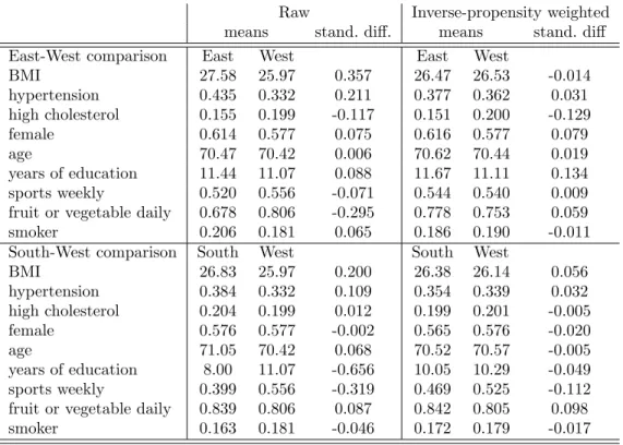
Finally, we evaluate the fit of the estimated causal forests in three ways. First, we check the overlap assumption by looking at whether the propensity scores are bounded away from zero and one. Second, we investigate covariate balance by comparing the inverse-propensity weighted averages of the explanatory variables across the two groups. (Here, treatment observations are weighted by 1/ˆpi and control observations by 1/(1−pˆi).) Third, we im- plement the “best linear predictor” method of Chernozhukov et al. [2018b]. In this method, motivated by equation (2), ˜Yi is regressed on Ci =τW˜i and Di = ˆτ(−i)(Xi)−τW˜i,where ˆ
τ(−i)(Xi) is the out-of-bag treatment effect estimate and τ is its sample average. If the coefficent of Ci is one then the model captures the average treatment effect adequately, and if the coefficient ofDi is one (or at least significantly positive) then the heterogeneity of the treatment effect is well calibrated, too. (See Athey and Wager [2019] for more details.)
4 Results
4.1 Prevalence
Figure 1a and the first column of Table 2 show unadjusted (raw) differences in diabetes prevalence across countries and regions, respectively, referring to the population aged at least 50 years as sampled in SHARE. Prevalence is significantly higher than average in Poland, the Czech Republic and Spain, and lower in Switzerland, Denmark, Austria, France, Belgium and Sweden. Taken the countries together, the prevalence exceeds the Western European average (12.7%) by 7.7% points in Eastern and by 5.7% points in Southern Europe.
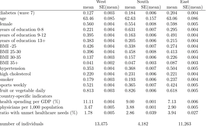
Descriptive statistics in Table 1 show that, compared to the Western European popu- lation, Eastern Europeans on average have less education, have a higher BMI (particularly in the obese and severely obese range), are more often diagnosed with hypertension, smoke more often; but play sports at least weekly or eat fruit or vegetable daily in a smaller propor- tion. Southern Europeans have less education, have a higher BMI (in the overweight range) and less often play sports than Western Europeans, but otherwise the differences are smaller than in the East-West dimension.
Looking at the country-specific indicators, health spending per GDP and the density of physicians are lower, while the prevalence of unmet needs is higher in the East than in the West. In the South, these indicators are in between, apart from the number of physicians, which is the highest there.
According to Table 2, the unadjusted East-West difference of 7.7 %points (odds ratio [OR]
= 1.76) is only slightly reduced by controlling for socio-economic variables (age, gender and years of education) but decreases to less than half (to 3.1 %points, OR=1.31) by controlling
further for health-related factors (BMI, hypertension, high cholesterol and lifestyle). The South-West difference decreases by more than one third, from 5.7% points to 3.4 %points (OR from 1.55 to 1.35) after controlling for the variables. According to Figure 1a, the unadjusted and adjusted differences differ only slightly on the country level, apart from Switzerland, Denmark and Austria, where a substantial portion of the better than average prevalence is explained by the favourable distribution of the risk factors.
However, as columns (4) and (8) in Table 2 indicate, once we add the three country- specific indicators to the regression (health spending per GDP, physicians per capita, preva- lence of unmet needs), the regional differences in diabetes prevalence disappear. Thus, differences in healthcare availability largely explain the residual differences in prevalence.
4.2 Incidence
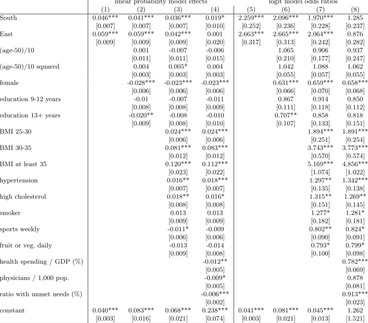
In the following, we focus on incidence (i.e. on the transition to diabetes) because risk factors measured before the diagnosis are more plausibly exogenous. Figure 1b and the first column of Table 3 show how the transition rate from non-diabetes to diabetes between waves 4 and 7 differs across countries and regions. Incidence is significantly higher than average in Hungary, Spain, Poland, the Czech Republic, and lower in Denmark, Switzerland, France, Germany, Sweden and Austria. Six-year incidence is by 5.9 %points (OR = 2.66) higher in Eastern and by 4.6 %points (OR = 2.26) higher in Southern Europe than in Western Europe (4.0%). According to Table 3, controlling for the socio-economic and health-related variables at wave 4 reduces the East-West difference to 4.2 %points (OR = 2.06) and the South-West difference to 3.6 %points (OR = 1.97).
Among the control variables, the three additional health-related components of the metabolic syndrome all increase the rate of transition to overt diabetes. Even overweight (25≤BM I <30),which characterises more than 40% of the 50+ population, is a significant risk factor (OR = 1.9), while the two classes of obesity have a markedly larger effect (OR
= 3.7 and 5.2, not significantly different from each other). Previous hypertension and high blood cholesterol have ORs around 1.3. Female gender is associated with strongly reduced diabetes incidence, while measured lifestyle factors have only marginally significant effects.
Just as in the case of diabetes prevalence, the bulk of the remaining regional differences in diabetes incidence is explained by the three country-specific healthcare indicators (columns (4) and (8) of Table 3).
4.3 Heterogeneity in incidence
The descriptive plots of Figure 2 show that hypertension, high blood cholesterol and high BMI are associated with a higher probability of new diabetes diagnosis in all three regions, but to varying degrees. For instance, the association of hypertension and high cholesterol with the diagnosis seems to be more pronounced in Eastern Europe than elsewhere.
To analyse the heterogeneity of regional effects, we train causal forests as explained in section 3.2. The causal forests yield very similar estimates for the average adjusted regional differences in diabetes incidence as the controlled linear probability model in Table 3: 3.8
%points (S.E. = 0.6 %point) for the East-West difference and 3.9 %points (S.E.= 0.4 %point) for the South-West difference. However, the value added of the causal forest approach is that it automatically yields effect estimates for each individual, so that they can be aggregated
by different risk factors.
The subsample-specific average treatment effects (calculated from equation 4), their 95%
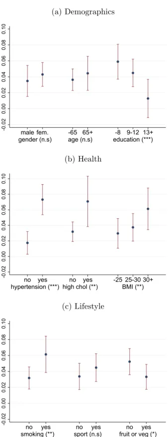
confidence intervals and the statistical significance of the between-group variations are dis- played in Figures 3–4. The adjusted East-West difference is significantly higher for individu- als with lower education level, with previous hypertension or high cholesterol and with higher BMI (especially with obesity), in such a way that the least vulnerable groups have essentially no excess transition risk to diabetes in the East compared to the West. For instance, the effect estimate is 1.3 %point (not significantly different from zero at the 10% level) for those with more than 12 years of schooling but 5.9 %points for those with at most 8 years, or 1.7
%points (not significantly different from zero at the 1% level) for those without hypertension and 7.3 %points for those with it. Among the lifestyle factors, smoking increases the excess risk significantly. Meanwhile, effect heterogeneity is not significant across gender, age or weekly sports activity.
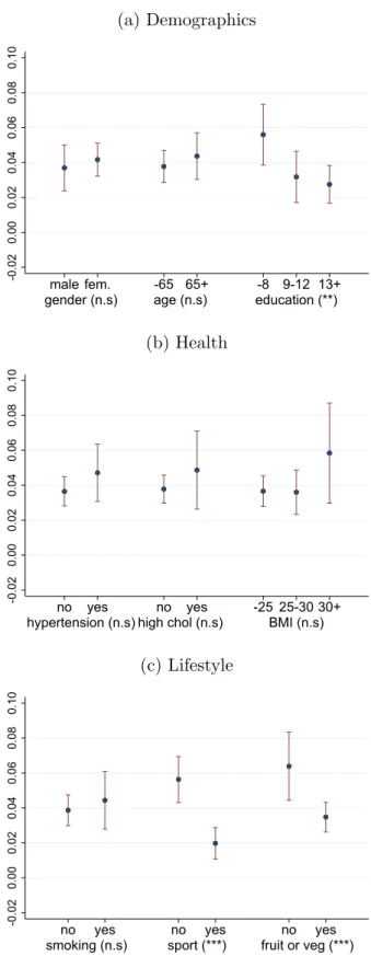
Overall, heterogeneity is much less pronounced in the South-West dimension (Figure 4), where the effect estimate is statistically significantly positive in each subsample. Here, lifestyle factors play a larger role in distinguishing between groups of low and high excess risk since weekly sports activity and daily fruit or vegetable consumption both decrease diabetes incidence.
The Appendix contains the goodness-of-fit analysis of the estimated causal forests. Ac- cording to Figure A1, the propensity scores are between 0.05 and 0.95, hence the overlap assumption holds both for the East-West and the South-West model. Table A1 shows that the large (standardized) differences in the explanatory variables (especially in BMI, hyper- tension and daily fruit or vegetable consumption in the East-West dimension; and BMI,
education and weekly sports activity in the South-West dimension) are substantially re- duced after weighting with the inverse of the propensity score, which points to a reasonable post-estimation balance across the explanatory variables. In fact, for most variables, the absolute value of the inverse-propensity weighted standardized difference is below 0.10, the threshold of appropriate balance as suggested by Austin [2009].
Finally, Table A2 displays the results of the “best linear prediction” method of Cher- nozhukov et al. [2018b]. For the East-West model, both coefficients are close to (and statis- tically not significantly different from) one, suggesting an appropriate fit both in terms of the average treatment effect and treatment effect heterogeneity. Meanwhile, for the South-West model, the coefficient of the average effect is essentially one, but the coefficient of effect heterogeneity takes an imprecisely estimated negative value (which is statistically not signif- icantly different either from zero or one). In line with Figure 4, this also suggests a roughly homogeneous treatment effect in the South-West dimension.6
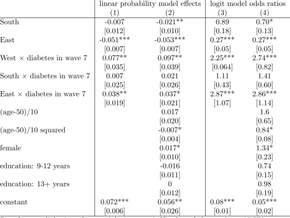
4.4 Management
Finally, we analyse how the new diagnosis of diabetes is associated with changes in dietary habits. Table 4 indicates that among the overweight population in wave 4 who remained non-diabetic throughout waves 4−7, weight loss due to diet in wave 7 was less prevalent by 5.1 %points in Eastern Europe than in Western Europe (OR = 0.27), while there was no difference in the South-West dimension. Compared to this population, the diagnosis of diabetes increased the prevalence of weight loss in the West (by 7.7 %points) as well as
6We tried various other specifications for the causal forest such as using the baseline built-in parameters or tuning only a subset of the parameters, but the conclusions did not change.
in the East (by 3.8 %points), while there was no change in the South. These results are essentially the same if control variables are included in the analysis. Hence, in Western, as well as in Eastern Europe, a new diabetes diagnosis is associated with a substantially increased likelihood of weight loss due to diet but no such association is found in the South.
5 Conclusions
Using data from three regions and 15 countries in Europe, we documented that diabetes prevalence and incidence are much higher in the South and East than in the West, and only 20−60% of these differences disappear by controlling for individual-level demographic and socio-economic characteristics, health status and health behaviour. The country-specific indicators of health spending, availability of physicians and prevalence of unmet needs explain the remaining part. Thus, the observed regional differences are likely to be caused by a combination of the differences in healthcare systems and in individual socio-economic and health-related variables.
Heterogeneity analyses showed that the East-West difference in incidence is essentially zero for the least vulnerable groups such as those with tertiary education or without hy- pertension. At the same time, Western European countries fare much better in preventing diabetes among lower-educated individuals, among those with comorbidities or with higher BMI. Meanwhile, the South-West difference seems more stable across these dimensions.
Using an indicator of change in dietary habits, we found that overweight individuals are less likely to change diet effectively in the South and East than in the West. However, among people newly diagnosed with diabetes, the prevalence of weight loss due to diet is similar in
the East and in the West. Thus, at least for the East, we do not see evidence that the higher incidence of diabetes would be coupled with worse management as measured by weight loss due to diet.
The analysis is subject to some limitations. First, the three examined regions are not homogeneous, thus, by construction, any regional analysis overlooks the differences across countries within a region. (Meanwhile, the country-level sample sizes are generally too small to yield powerful conclusions.) Second, we could only use a crude measure of diabetes management – weight loss due to diet. Unfortunately we observe neither the respondents’
participation in laboratory tests (blood glucose or glycated hemoglobin [HbA1c] measure- ments) nor their blood sample results. Also, while we observe the raw number of doctoral visits, further details on outpatient care are not available. Third, all of our estimates refer to diagnosed diabetes, although undiagnosed cases make up one-third to one-half of total (diagnosed and undiagnosed) prevalence [IDF, 2019]. In the future, the analysis of blood samples taken within the SHARE survey may facilitate further cross-country comparisons of both diabetes management and the prevalence of undiagnosed diabetes.
Overall, our results suggest that in Eastern Europe, more emphasis should be put on the prevention of diabetes among individuals more prone to the disease, which could at least partly be achieved by interventions aimed at preventing obesity, hypertension or high cholesterol among the high-risk population.
References
E. Agardh, P. Allebeck, J. Hallqvist, T. Moradi, and A. Sidorchuk. Type 2 diabetes incidence and socio-economic position: A systematic review and meta-analysis. International Jour- nal of Epidemiology, 40(3):804–818, 2011. URLhttps://doi.org/10.1093/ije/dyr029.
S. Athey and S. Wager. Estimating treatment effects with causal forests: An application.
Observational Studies, 5:36–51, 2019. URL https://obsstudies.org/277-2/.
S. Athey, J. Tibshirani, and S. Wager. Generalized random forests. The Annals of Statistics, 47(2):1148–1178, 2019. URL https://doi.org/10.1214/18-AOS1709.
P. C. Austin. Using the standardized difference to compare the prevalence of a binary variable between two groups in observational research. Communications in Statistics - Simulation and Computation, 38(6):1228–1234, 2009. URL https://doi.org/10.1080/
03610910902859574.
O. Bashkin, R. Horne, and I. P. Bridevaux. Influence of health status on the association between diabetes and depression among adults in Europe: Findings from the SHARE international survey. Diabetes Spectrum, 31(1):75–82, 2018. URL https://doi.org/10.
2337/ds16-0063.
A. B¨orsch-Supan. Survey of Health, Ageing and Retirement in Europe (SHARE) wave 7.
Release version: 7.0.0., 2019. URLhttps://doi.org/10.6103/SHARE.w7.700. Accessed:
2019-05-02.
A. B¨orsch-Supan, M. Brandt, C. Hunkler, T. Kneip, J. Korbmacher, F. Malter, B. Schaan,
S. Stuck, and S. Zuber. Data resource profile: the Survey of Health, Ageing and Retirement in Europe (SHARE). International Journal of Epidemiology, 42(4):992–1001, 2013. URL https://doi.org/10.1093/ije/dyt088.
V. Chernozhukov, D. Chetverikov, M. Demirer, E. Duflo, C. Hansen, W. Newey, and J. Robins. Double/debiased machine learning for treatment and structural parame- ters. The Econometrics Journal, 21(1):C1–C68, 2018a. URLhttps://doi.org/10.1111/
ectj.12097.
V. Chernozhukov, M. Demirer, E. Duflo, and I. Fernandez-Val. Generic machine learning inference on heterogenous treatment effects in randomized experiments. Working Paper 24678, National Bureau of Economic Research, 2018b. URL https://www.nber.org/
papers/w24678.
A. Espelt, C. Borrell, L. Pal`encia, A. Goday, T. Spadea, R. Gnavi, L. Font-Ribera, and A. E. Kunst. Socioeconomic inequalities in the incidence and prevalence of type 2 diabetes mellitus in Europe. Gaceta Sanitaria, 27(6):494–501, 2013. URLhttps://doi/10.1016/
j.gaceta.2013.03.002.
Eurostat. Eurostat database, population and social conditions, health, health care, 2020.
URLhttps://ec.europa.eu/eurostat/data/database. Accessed: 2020-04-04.
M. H. Farrell. Robust inference on average treatment effects with possibly more covariates than observations. Journal of Econometrics, 189(1):1–23, 2015. URLhttps://doi.org/
10.1016/j.jeconom.2015.06.017.
T. Hastie, R. Tibshirani, and J. Friedman. The Elements of Statistical Learning. Springer Series in Statistics. Springer New York Inc., New York, NY, USA, 2009.
I. Huang, M. A. Lim, and R. Pranata. Diabetes mellitus is associated with increased mortality and severity of disease in COVID-19 pneumonia - A systematic review, meta-analysis, and meta-regression.Diabetes & Metabolic Syndrome: Clinical Research & Reviews, 14(4):395–
403, 2020. ISSN 1871-4021. URLhttps://doi.org/10.1016/j.dsx.2020.04.018.
IDF. Diabetes Atlas 9th edition. https://diabetesatlas.org/en/resources/, 2019. Ac- cessed: 2019-12-12.
E. Kassi, P. Pervanidou, G. Kaltsas, and G. Chrousos. Metabolic syndrome: defini- tions and controversies. BMC Medicine, 9:48, 2011. URL https://doi.org/10.1186/
1741-7015-9-48.
W. C. Knowler, E. Barrett-Connor, S. E. Fowler, R. F. Hamman, J. M. Lachin, E. A. Walker, and D. M. Nathan. Reduction in the incidence of type 2 diabetes with lifestyle intervention or metformin. The New England Journal of Medicine, 346(6):393–403, 2002.
T. Kouwenhoven-Pasmooij, A. Burdorf, J. Roos-Hesselink, M. Hunink, and S. Robroek.
Cardiovascular disease, diabetes and early exit from paid employment in Europe; the impact of work-related factors. International Journal of Cardiology, 215:332–337, 2016.
ISSN 0167-5273. URLhttps://doi.org/10.1016/j.ijcard.2016.04.090.
S. Li, J. Wang, B. Zhang, X. Li, and Y. Liu. Diabetes mellitus and cause-specific mortality:
A population-based study. Diabetes & Metabolism Journal, 43(3):319–341, 2019. URL https://doi.org/10.4093/dmj.2018.0060.
F. Malter and A. B¨orsch-Supan. SHARE wave 5: Innovations & methodology. Technical report, Munich: MEA at the Max Planck Institute for Social Law and Social Policy, 2015. URL http://www.share-project.org/fileadmin/pdf_documentation/Method_
vol5_31March2015.pdf.
K. V. Narayan, J. P. Boyle, T. J. Thompson, E. W. Gregg, and D. F. Williamson. Effect of BMI on lifetime risk for diabetes in the US. Diabetes Care, 30(6):1562–1566, 2007.
B. Rodriguez-Sanchez and D. Cantarero-Prieto. Socioeconomic differences in the associations between diabetes and hospital admission and mortality among older adults in Europe.
Economics and Human Biology, 33:89–100, 2019. URL https://doi.org/10.1016/j.
ehb.2018.12.007.
J. Rumball-Smith, D. Barthold, A. Nandi, and J. Heymann. Diabetes associated with early labor-force exit: A comparison of sixteen high-income countries. Health Affairs, 33(1):
110–115, 2014. URLhttps://doi.org/10.1377/hlthaff.2013.0518.
T. Tamayo, J. Rosenbauer, S. Wild, A. Spijkerman, C. Baan, N. Forouhi, C. Herder, and W. Rathmann. Diabetes in Europe: An update. Diabetes Research and Clinical Practice, 103(2):206–217, 2014. URLhttps://doi.org/10.1016/j.diabres.2013.11.007.
J. Tibshirani, S. Athey, and S. Wager. grf: Generalized Random Forests, 2019. URL https:
//CRAN.R-project.org/package=grf. R package version 0.10.4.
S. Wager and S. Athey. Estimation and inference of heterogeneous treatment effects using random forests. Journal of the American Statistical Association, 113(523):1228–1242, 2018. URLhttps://doi.org/10.1080/01621459.2017.1319839.
D. R. Whiting, L. Guariguata, C. Weil, and J. Shaw. IDF Diabetes Atlas: Global estimates of the prevalence of diabetes for 2011 and 2030. Diabetes Research and Clinical Practice, 94(3):311–321, 2011. URLhttps://doi.org/10.1016/j.diabres.2011.10.029.
WHO. European Health Information Gateway, Physicians per 100 000, 2020. URL https:
//gateway.euro.who.int/en/indicators/hfa_494-5250-physicians-per-100-000/.
Accessed: 2020-04-04.
Tables and figures
West South East
mean SE(mean) mean SE(mean) mean SE(mean)
diabetes (wave 7) 0.127 0.003 0.184 0.006 0.204 0.004
age 63.46 0.085 62.63 0.157 63.06 0.086
female 0.560 0.004 0.554 0.008 0.598 0.005
years of education 0-8 0.221 0.004 0.631 0.007 0.295 0.004
years of education 9-12 0.395 0.004 0.163 0.006 0.491 0.004
years of education 13+ 0.383 0.004 0.205 0.006 0.215 0.004
BMI -25 0.426 0.004 0.338 0.007 0.274 0.004
BMI 25-30 0.396 0.004 0.458 0.008 0.413 0.005
BMI 30-35 0.137 0.003 0.157 0.006 0.226 0.004
BMI 35+ 0.041 0.002 0.047 0.003 0.087 0.003
hypertension 0.353 0.004 0.368 0.007 0.504 0.005
high cholesterol 0.220 0.004 0.231 0.006 0.221 0.004
smoker 0.179 0.003 0.193 0.006 0.237 0.004
sports weekly 0.521 0.004 0.365 0.007 0.424 0.005
fruit or vegetable daily 0.813 0.003 0.826 0.006 0.618 0.005
country-specific indicators
health spending per GDP (%) 11.11 0.004 9.00 0.001 7.13 0.006
physicians per 1,000 population 3.47 0.005 3.88 0.001 2.90 0.005 ratio with unmet healthcare needs (%) 1.78 0.005 2.86 0.039 3.94 0.027
number of individuals 13,475 4,182 11,263
Apart from wave 7 diabetes, all indicators are measured in wave 4.
Table 1: Descriptive statistics of the variables used in Table 2
(a) Prevalence
-0.10-0.050.000.050.10 Switzerland Denmark Austria France Belgium Sweden Estonia Italy Germany Slovenia Hungary Portugal Spain Czech Republic Poland
unadjusted adjusted
(b) Incidence
-0.050.000.050.10 Denmark Switzerland France Germany Sweden Austria Belgium Portugal Italy Estonia Slovenia Czech Republic Poland Spain Hungary
unadjusted adjusted
Figure 1: Unadjusted and adjusted diabetes prevalence and incidence by countries, deviations from the mean. Adjustment is made by controlling for the individual-specific variables listed in Tables 2–3.
linear probability model effects logit model odds ratios
(1) (2) (3) (4) (5) (6) (7) (8)
South 0.057*** 0.045*** 0.034*** 0.007 1.553*** 1.415*** 1.354*** 1.023
[0.010] [0.009] [0.009] [0.014] [0.113] [0.101] [0.103] [0.122]
East 0.077*** 0.070*** 0.031*** -0.014 1.760*** 1.689*** 1.313*** 0.840
[0.011] [0.010] [0.010] [0.026] [0.127] [0.121] [0.099] [0.174]
(age-50)/10 0.075*** 0.036** 0.050*** 1.942*** 1.450*** 1.672***
[0.015] [0.014] [0.019] [0.270] [0.204] [0.309]
(age-50)/10 squared -0.013*** -0.006 -0.007 0.884*** 0.941* 0.932*
[0.004] [0.004] [0.004] [0.033] [0.035] [0.034]
female -0.043*** -0.040*** -0.041*** 0.719*** 0.703*** 0.693***
[0.009] [0.008] [0.008] [0.046] [0.048] [0.047]
education 9-12 years -0.026** -0.017* -0.029** 0.849** 0.895 0.814**
[0.011] [0.010] [0.011] [0.066] [0.073] [0.070]
education 13+ years -0.060*** -0.026** -0.043*** 0.616*** 0.780*** 0.655***
[0.011] [0.011] [0.013] [0.055] [0.074] [0074]
BMI 25-30 0.052*** 0.050*** 1.855*** 1.816***
[0.008] [0.008] [0.160] [0.157]
BMI 30-35 0.157*** 0.156*** 3.564*** 3.521***
[0.014] [0.014] [0.347] [0344]
BMI at least 35 0.286*** 0.282*** 6.514*** 6.337***
[0.025] [0.025] [0.839] [0.825]
hypertension 0.064*** 0.065*** 1.633*** 1.654***
[0.009] [0.009] [0.114] [0.114]
high cholesterol 0.088*** 0.087*** 1.810*** 1.797***
[0.011] [0.011] [0.130] [0.129]
smoker 0.014 0.012 1.157 1.138
[0.011] [0.011] [0.111] [0.109]
sports weekly -0.043*** -0.040*** 0.683*** 0.705***
[0.008] [0.008] [0.049] [0.050]
fruit or veg. daily -0.01 -0.010 0.907 0.915
[0.011] [0.011] [0.077] [0.078]
health spending / GDP (%) -0.015** 0.867***
[0.007] [0.048]
physicians / 1,000 pop. -0.005 0.959
[0.007] [0.059]
ratio with unmet needs (%) -0.008*** 0.937***
[0.002] [0.016]
constant 0.127*** 0.162*** 0.106*** 0.285*** 0.146*** 0.171*** 0.092*** 0.460
[0.003] [0.016] [0.021] [0.094] [0.003] [0.021] [0.013] [0.358]
Number of observations: 28,920. All explanatory variables are measured in wave 4.
Standard errors in brackets (OLS: robust), *** p<0.01, ** p<0.05, * p<0.1
Table 2: OLS and logit models of diabetes prevalence in SHARE wave 7
linear probability model effects logit model odds ratios
(1) (2) (3) (4) (5) (6) (7) (8)
South 0.046*** 0.041*** 0.036*** 0.019* 2.259*** 2.096*** 1.970*** 1.285
[0.007] [0.007] [0.007] [0.010] [0.252] [0.236] [0.228] [0.237]
East 0.059*** 0.059*** 0.042*** 0.001 2.663*** 2.665*** 2.064*** 0.876
[0.009] [0.009] [0.009] [0.020] [0.317] [0.313] [0.242] [0.282]
(age-50)/10 0.001 -0.007 -0.006 1.065 0.906 0.937
[0.011] [0.011] [0.015] [0.210] [0.177] [0.247]
(age-50)/10 squared 0.004 0.005* 0.004 1.042 1.088 1.062
[0.003] [0.003] [0.003] [0.055] [0.057] [0.055]
female -0.028*** -0.023*** -0.023*** 0.631*** 0.659*** 0.658***
[0.006] [0.006] [0.006] [0.066] [0.070] [0.068]
education 9-12 years -0.01 -0.007 -0.011 0.867 0.914 0.850
[0.008] [0.008] [0.009] [0.111] [0.118] [0.112]
education 13+ years -0.020** -0.008 -0.010 0.707** 0.858 0.818
[0.009] [0.008] [0.010] [0.107] [0.133] [0.151]
BMI 25-30 0.024*** 0.024*** 1.894*** 1.891***
[0.006] [0.006] [0.251] [0.254]
BMI 30-35 0.081*** 0.083*** 3.743*** 3.773***
[0.012] [0.012] [0.570] [0.574]
BMI at least 35 0.120*** 0.112*** 5.169*** 4.856***
[0.023] [0.022] [1.074] [1.022]
hypertension 0.016** 0.018*** 1.297** 1.342***
[0.007] [0.007] [0.135] [0.138]
high cholesterol 0.018** 0.016* 1.315** 1.269**
[0.008] [0.008] [0.151] [0.145]
smoker 0.013 0.013 1.277* 1.281*
[0.009] [0.009] [0.182] [0.181]
sports weekly -0.011* -0.009 0.802** 0.824*
[0.006] [0.006] [0.090] [0.091]
fruit or veg. daily -0.013 -0.014 0.793* 0.799*
[0.009] [0.008] [0.100] [0.098]
health spending / GDP (%) -0.012** 0.782***
[0.005] [0.069]
physicians / 1,000 pop. -0.009* 0.878
[0.005] [0.081]
ratio with unmet needs (%) -0.006*** 0.913***
[0.002] [0.023]
constant 0.040*** 0.083*** 0.068*** 0.238*** 0.041*** 0.081*** 0.045*** 1.262
[0.003] [0.016] [0.021] [0.074] [0.003] [0.021] [0.013] [1.521]
Number of observations: 25,155. All explanatory variables are measured in wave 4.
Standard errors in brackets (OLS: robust), *** p<0.01, ** p<0.05, * p<0.1
Table 3: OLS and logit models of new diabetes diagnosis between SHARE waves 4 and 7
(a) by hypertension in wave 4
0.000.050.100.15
West South East
non-hypertensive hypertensive
(b) by high cholesterol in wave 4
0.000.050.100.150.20
West South East
not high cholesterol high cholesterol
(c) by BMI category in wave 4
0.000.050.100.150.200.250.30
West South East
normal BMI BMI 25-30
BMI 30-35 BMI 35-
Figure 2: Transition probabilities to diabetes between SHARE waves 4 and 7, by hyperten- sion, high cholesterol and BMI category measured in wave 4
(a) Demographics
-0.020.000.020.040.060.080.10
gender (n.s)male fem. age (n.s)-65 65+ education (***)-8 9-12 13+
(b) Health
-0.020.000.020.040.060.080.10
hypertension (***) high chol (**)no yes no yes -25 25-30 30+BMI (**)
(c) Lifestyle
-0.020.000.020.040.060.080.10
smoking (**)no yes sport (n.s)no yes fruit or veg (*)no yes
Figure 3: Average individual-level adjusted East-West differences (average treatment ef- fects, ATE) by various risk factors, with 95% confidence intervals and with the statistical significance of the between-group variation (*** p<0.01, ** p<0.05, * p<0.1, n.s p≥0.1)
(a) Demographics
-0.020.000.020.040.060.080.10
gender (n.s)male fem. age (n.s)-65 65+ education (**)-8 9-12 13+
(b) Health
-0.020.000.020.040.060.080.10
hypertension (n.s) high chol (n.s)no yes no yes -25 25-30 30+BMI (n.s)
(c) Lifestyle
-0.020.000.020.040.060.080.10
smoking (n.s)no yes sport (***)no yes fruit or veg (***)no yes
Figure 4: Average individual-level adjusted South-West differences (average treatment ef- fects, ATE) by various risk factors, with 95% confidence intervals and with the statistical significance of the between-group variation (*** p<0.01, ** p<0.05, * p<0.1, n.s p≥0.1)
linear probability model effects logit model odds ratios
(1) (2) (3) (4)
South -0.007 -0.021** 0.89 0.70*
[0.012] [0.010] [0.18] [0.13]
East -0.051*** -0.053*** 0.27*** 0.27***
[0.007] [0.007] [0.05] [0.05]
West×diabetes in wave 7 0.077** 0.097** 2.25*** 2.74***
[0.035] [0.039] [0.064] [0.82]
South×diabetes in wave 7 0.007 0.021 1.11 1.41
[0.025] [0.026] [0.43] [0.60]
East×diabetes in wave 7 0.038** 0.037* 2.87*** 2.86***
[0.019] [0.021] [1.07] [1.14]
(age-50)/10 0.017 1.6
[0.020] [0.65]
(age-50)/10 squared -0.007* 0.84*
[0.004] [0.08]
female 0.017* 1.34*
[0.010] [0.23]
education: 9-12 years -0.016 0.74
[0.011] [0.15]
education: 13+ years 0 0.98
[0.012] [0.19]
constant 0.072*** 0.056** 0.08*** 0.05***
[0.006] [0.026] [0.01] [0.02]
Sample: non-diabetic and overweight in wave 4. Number of observations: 10,574.
The explanatory variables are measured in wave 4, apart from diabetes in wave 7.
Standard errors in brackets (OLS: robust). *** p<0.01, ** p<0.05, * p<0.1.
Table 4: Models of the probability of reporting weight loss due to diet in SHARE wave 7
Appendix
A Goodness-of-fit analysis of the estimated causal forests
propensity score
Density
0.0 0.2 0.4 0.6 0.8 1.0
0.00.51.01.52.0
(a) East-West model
propensity score
Density
0.0 0.2 0.4 0.6 0.8 1.0
01234
(b) South-West model Figure A1: Histogram of the propensity scores in the causal forest models