analyses Regional differences in diabetes across Europe – regression and causalforest Economics and Human Biology

(1)

Regional differences in diabetes across Europe – regression and causal forest analyses

Péter Elek

^a,b,c,

*, Anikó Bíró

^a

aHealthandPopulation“Lendület”ResearchGroup,CentreforEconomicandRegionalStudies,Budapest,Hungary

bInstituteofEconomics,CorvinusUniversityofBudapest,Hungary

cDepartmentofEconomics,EötvösLorándUniversity(ELTE),Budapest,Hungary

ARTICLE INFO Articlehistory:

Received8July2020

Receivedinrevisedform4November2020 Accepted10November2020

Availableonline12November2020 JELclassiﬁcation:

C21 C45 I10 I12 I14 Keywords:

Causalforest Diabetes Europe Healthbehaviour SHAREdata

ABSTRACT

WeexamineregionaldifferencesindiabeteswithinEurope,and relatethemtovariationsinsocio- economicconditions,comorbidities,healthbehaviouranddiabetesmanagement.WeusetheSHARE (Survey of Health, Ageingand Retirementin Europe) data of 15 European countries and 28,454 individuals,whoparticipatedbothinthe4thand7th(year2011and2017)wavesofthesurvey.First,we estimate multivariate regressions, where the outcome variables are diabetes prevalence,diabetes incidence, and weight loss due to diet as an indicator of management. Second, we study the heterogeneousimpactofdemographic,socio-economic,healthandlifestyleindicatorsontheregional differencesindiabetesincidencewithcausalrandomforests.

ComparedtoWesternEurope,theoddsofanewdiabetesdiagnosisoverasix-yearhorizonis2.2-fold higherinSouthernand2.6-foldhigherinEasternEurope.Adjustingforindividualcharacteristics,the oddsratiodecreasesto1.8intheSouth-Westandto2.0intheEast-Westdimension.Theseremaining differencesaremostlyexplainedbycountry-speciﬁchealthcareindicators.Basedonthecausalforest approach, theadjustedEast-Westdifferenceis essentiallyzeroforthelowest riskgroups (tertiary education,employment,nohypertension,nooverweight)andincreasessubstantiallywiththeserisk factors,buttheSouth-Westdifferenceismuchlessheterogeneous.Theprevalenceofdiet-relatedweight lossaroundthetimeofdiagnosisalsoexhibitsregionalvariation.Theresultssuggestthattheregional differencesindiabetesincidencecouldbereducedbyputtingmoreemphasisondiabetesprevention amonghigh-riskindividualsinEasternandSouthernEurope.

1.Introduction

Livingwithdiabetesmellitusisassociatedwithincreasedall- causemortalityaswellasmortalityduetocardiovasculardisease, chronic lower respiratory diseases, inﬂuenza, pneumonia, and kidneydisease(Lietal.,2019).Morerecently,diabeteshasbeen showntoincreasethemortalityrateandtheprogressiontosevere diseaseinCOVID-19aroundtwofold(Huangetal.,2020).

Inthispaper,ouraimistodocumentregionaldifferencesinthe prevalenceandincidenceofdiabetesacrossEurope,andtorelate these differences to variations in socio-economic conditions, comorbidities, health behaviour and diabetes management.

Around 8.9%of Europeansaged 20-79yearslive withdiabetes, and 8.5% of all deaths is attributable to diabetes and its complications (IDF, 2019).However,theregionaldistribution is

veryuneven:prevalenceshowsamorethantwofoldandmortality amorethanfourfolddifferenceevenacrossthememberstatesof theEuropean Union (Whiting etal.,2011; IDF,2019).It is well knownthatgenetics,lifestyle,dietandthehealthcaresystemall inﬂuencetheincidenceandmortalityindiabetes,andtheserisk factorsareunevenlydistributedacrossthepopulationofEuropean countries(Tamayoetal.,2014).Inparticular,therolesofsocio- economicinequalities(Agardhetal.,2011;Espeltetal.,2013),of thebody massindex(e.g.Narayan etal., 2007)and oflifestyle changes(e.g.DiabetesPreventionProgramResearchGroup,2002) arewelldocumented.However,lessisknownabouttherelative roleofthesefactorsinexplainingthevariationofdiabetesacross Europe.Ourstudyaimstoﬁllthisgap.

The risk factorsfor diabetes are highly correlated and may inﬂuencediabetes prevalenceand incidencein a nonlinearand non-additive way. For instance, the combination of obesity, hypertension,slightlyelevatedbloodsugarandabnormalcholes- terollevelmarkedlyincreasestheriskofcardiovasculardisease and the transition rate toovert diabetes. This is the rationale

*Correspondingauthor.1097Budapest,TóthKálmánutca4.,Hungary.

E-mailaddresses:elek.peter@krtk.hu(P.Elek),biro.aniko@krtk.hu(A.Bíró).

http://dx.doi.org/10.1016/j.ehb.2020.100948

).

ContentslistsavailableatScienceDirect

Economics and Human Biology

j o u r n a lh o m e p ag e : w w w . e l s e vi e r . c o m / l o c a t e/ e h b

(2)

behindthediagnosisofthemetabolicsyndrome,whichisdefined, roughly,whenapatienthasatleastthreeriskfactorsoutofthe abovefour.Somestudiesarguethatmetabolicsyndromeismore thanitspartsintermsofcardiovascularorovertdiabetesrisk(but seee.g.Kassietal.,2011forareviewofcontroversies),suggesting interaction effects between the risk factors. We train a causal randomforestdevelopedbyWagerandAthey(2018)and Athey etal.(2019)toinvestigateheterogeneityintheadjustedregional differencesindiabetesincidence.Specifically,weanalysehowthe regionaldifferencesin diabetesincidencevarybydemographic, socio-economic, health and lifestyle indicators. Compared to a traditional full interaction linear regression model, the main benefitofthecausalforestmethodisthegaininstatisticalpower duetotheautomatedchoiceofheterogeneitiestobeincludedin the model. Finally, we investigate regional differences in the changeinhealthbehaviour(theprobabilityofweightlossdueto diet)aroundthetimeofdiabetesdiagnosis.Theresultsshedlight ontheoriginsofthemarkedcross-countrydifferencesindiabetes throughoutEurope.

WeusetheSurveyofHealth,AgeingandRetirementinEurope (SHARE)(Börsch-Supan,2019).SHAREisacross-nationalEuropean panel databaseof micro dataondemographic, socio-economic, labourmarket,healthandlifestyleinformationofindividualsaged 50 or older, henceit is a convenientdatabase foranalysing all important diabetes-related factors simultaneously. Indeed, a numberofstudieshaveusedSHAREfordiabetesresearch.Based onSHARE data,Rodriguez-SanchezandCantarero-Prieto (2019) showapositiveassociationofdiabeteswithhospitaladmissions anddeath,whileEspeltetal.(2013)findthateducationisinversely associated with diabetes prevalence and (for women) with diabetes incidence. Diabetes is known to increase the rate of labourforceexitbyaround30%(Rumball-Smithetal.,2014)and theprobabilityofdisabilitybenefitsmorethantwofold(Kouwen- hoven-Pasmooijetal.,2016).Bashkinetal.(2018)alsouseSHARE datatoshowthatthepositiveassociationbetweendiabetesand depressionisnolongersignificantafteradjustingforarichsetof individualcharacteristics.

Wemakeseveralcontributionstotheexistingliterature.First, beyond examining diabetes prevalence, we also analyse the transitiontodiabetesoverasix-yearhorizon,asufﬁcientlylong time period tomeasure theeffectof theexplanatory variables.

Second,weinvestigatehowtheprevalenceandincidencediffer- encesbetweenthethreeregionsofEuropevarybyindividualrisk factorsandapplythenovelcausalforestmethodologytoanswer this question. Finally, we relate weight loss – an indicator of diabetesmanagement–tothepatternsoftransitiontodiabetes.

2.Data

TheSHAREsurveyswereconductedinsevenwaves,startingin 2004,andthecurrentlylastwavewastakenin2017.¹Thenumber of participatingcountriesgraduallyexpanded from12 to27to includenewEUmemberstatesaswell.Weexploitthepanelnature

ofthesurveybyusingwaves4and7,whichweretakensixyears apart(2011and2017),hencetransitiontodiabetescanbereliably examinedonthem.Wesplitthe15countriesthatappearinboth wavesintothreegroups:West[includingNorth](Austria,Belgium, Denmark, France, Germany,Sweden, Switzerland); South (Italy, Portugal,Spain);East(CzechRepublic,Estonia,Hungary,Poland, Slovenia).² We usecalibratedweightstoavoidbias duetounit nonresponse and panelattrition (seeMalter andBörsch-Supan, 2015fordetails).

Inouranalysis,wetreatapersonashavingdiabetesifhe/she answered“yes”toanyofthefollowingtwoquestions:(1)“Hasa doctorevertoldyouthatyouhad/Doyoucurrentlyhavediabetes orhighbloodsugar?”(2)“Doyoucurrentlytakedrugsatleastonce aweekfordiabetesorhighbloodsugar?”Weexaminediabetes prevalence,i.e.thebinaryindicatorofhavingdiabetesinwave7;

and diabetes incidence (transition to diabetes), i.e. the binary indicatorofhavingdiabetesinwave7amongthosewhodidnot havediabetesinwave4.WedonotdistinguishbetweenType1and Type 2 diabetes, but around 90% of the prevalence and the overwhelmingmajorityofincidenceabove50yearsbelongstothe lattercategory(IDF,2019).

Other variables – which we use as explanatory variables – includeregion, demographicand socio-economiccharacteristics (gender,age,yearsofeducation,employmentstatus),bodymass index(BMI,calculatedfromself-reportedheightandweight,and then categorised into normal weight (BMI<25), overweight (25BMI<30), obesity(30BMI)³ and, as a subgroup, severe obesity(35BMI)),comorbidities(hypertensionandhighcholes- terol,measuredbydruguseontheseconditions,andhavingever beendiagnosedwithheartattackorstroke)andlifestylefactors (binaryindicatorsofsmokingnow;playingsportsatleastoncea week;eatingfruitsorvegetablesdaily).Weusetheexplanatory variablesfromwave4.Thedatasetalsocontainstheself-reported binaryindicatorofhavinglostweightduetodietduringthepast12 monthsinwave7.

Wemergethreecountry-speciﬁchealthcareindicatorstothe SHAREdata:totalhealthcarespendingperGDP(source:Eurostat, 2020);thenumber ofphysiciansper1,000 inhabitants(source:

WHO,2020);andtheshareofthepopulationaged16andabove whoreportunmetneedsformedicalcareduetoﬁnancialreasons, waitinglistsorhavingtotraveltoofar(source:Eurostat,2020).The indicatorsrefertoyear2011(thetimeofwave4),exceptforhealth spendingperGDP,whichreferstoyear2013(duetomissingdatain 2011). Our aim with these indicators is to capture healthcare availabilityandquality.Whilethenumberofphysiciansandthe prevalence of unmet needs are direct measures of healthcare availability, theindicatorof healthcare spending canserve asa proxy for healthcare quality due to its known relation to advancements in medical technology (Beilfuss and Thornton 2016; Newhouse,1992) and loweravoidable mortality (Heijink etal.,2013).

1ThispaperusesdatafromSHAREWaves1,2,3,4,5,6and7(DOIs:10.6103/

SHARE.w1.700, 10.6103/SHARE.w2.700, 10.6103/SHARE.w3.700, 10.6103/SHARE.

w4.700,10.6103/SHARE.w5.700,10.6103/SHARE.w6.700,10.6103/SHARE.w7.700), see Börsch-Supan et al. (2013) for methodological details. The SHARE data collectionhasbeenprimarilyfundedbytheEuropeanCommissionthroughFP5 (QLK6-CT-2001-00360),FP6(SHARE-I3:RII-CT-2006-062193,COMPARE:CIT5-CT- 2005-028857, SHARELIFE: CIT4-CT-2006-028812) and FP7 (SHARE-PREP:

No211909,SHARE-LEAP:No227822,SHAREM4:No261982).Additionalfunding fromtheGermanMinistryofEducationandResearch,theMaxPlanckSocietyfor theAdvancementofScience,theU.S.NationalInstituteonAging(U01_AG09740- 13S2,P01_AG005842,P01_AG08291,P30_AG12815,R21_AG025169,Y1-AG-4553- 01,IAG_BSR06-11,OGHA_04-064,HHSN271201300071C)andfromvariousnational fundingsourcesisgratefullyacknowledged(seewww.share-project.org).

2 Weusedatafromwaves4and7toensurethatatleastthreecountriesare presentfromeachregionandasufﬁcientnumberoftransitionstodiabetesis observed.Hungary,PolandandPortugalwerenotincludedinwave5,Hungarydid notappearinwave6,either.Usingdatafromwaves4and6,waves5and7orwaves 6and7wouldreducethenumberofobservedtransitionsby15%,17%and34%, respectively.Thevariationincountrycoverageandsurveycontenthindersusfrom conductingapanelanalysiswithmorethantwowaves.

3 Only1%oftherespondentsinwave4areunderweight(BMI<18.5),whomwe includeinthenormalweightcategory.

(3)

3.Methods

3.1.Multivariateregressions

We ﬁt linear probability and logit models on diabetes prevalence (i.e. being diabetic in wave 7) and incidence (i.e.

becoming diabetic between waves 4 and 7), respectively. We include gradually more control variables beyond the regional dummies (or in some speciﬁcations the country dummies) to examine their confounding effect on regional / cross-country differences. First, weadd thedemographic and socio-economic indicators (age, age squared, gender, education categories and employment). Then, we extend the models with indicators of healthstatus(BMIcategories,hypertension,highbloodcholester- ol)andhealthbehaviour(smoking,weeklysportsactivityanddaily fruitorvegetableconsumption).⁴Toreducetheproblemofreverse causalityontheindividuallevel,weusetheexplanatoryvariables fromwave4.Asthelastextension,weaddthecountry-speciﬁc healthcare indicators to the explanatory variables to check whethertheyexplaintheremainingpartofregionaldifferences.

Wealsoinvestigatethechangeinhealthbehaviouraroundthe timeofdiabetesdiagnosis.Speciﬁcally,weestimatelinearandlogit modelsoftheprobabilityofweightlossduetodietinwave7.Weﬁt thesemodelsonthesampleofindividualswhowerenotdiabeticin wave4,andusetheinteractionoftheregionaldummieswiththe wave 7 diabetes dummy (and other controls) to investigate regionalheterogeneitiesintheprevalenceofweightlossduetothe diagnosisofdiabetes.Asasupplementaryanalysis,tounderstand theco-movementofdiabetesdiagnosisandweightlossduetodiet, weaddwaves5and6oftheSHAREdatatooursample,lookatthe two-year transitions todiabetesfor theavailable countriesand analysetheprevalenceofweightlossduetodietconcurrently,as wellasoneortwowavesbeforeandoneortwowavesafterthe diagnosis(i.e.uptofouryearsbeforeandfouryearsafterit).

3.2.Causalforests

Inordertoanalysetheheterogeneouseffectoftheriskfactors ontheregionaldifferencesindiabetesincidence,wetraincausal forests separatelyonEast-Westand South-Westdifferences (in each analysis we omit the third category from the sample).

Speciﬁcally,letWibetheregionaldummy(whichtakesoneforEast or South and zerofor West)and Xidenote theindividual-level demographic,socio-economic,health-andlifestyle-relatedcontrol variables. Let Yið1Þ¼YiðWi¼1Þ and Yið0Þ¼YiðWi¼0Þ be the potentialoutcomes,i.e.thediabetesstatusofaparticularpersonin the(imagined) situationthatsheis inEastern(Southern)or in Western Europe, respectively. (We set Western Europe as the referencecategorybecausediabetesincidenceisthelowestthere.) Weseektoestimatetheconditional“treatment”effect

t

^ð^x^Þ^¼^E^ð^Yⁱ^ð¹^Þ^Yⁱ^ð⁰^ÞjXⁱ^¼^x^Þ

assuming unconfoundedness andoverlap. Theunconfoundedness assumption states that fYið1Þ;Yið0Þg are independent from Wi

conditionalonthevalueofX_i,whileoverlapmeansthat0<pðxÞ<

1; where pðxÞ¼ Pr ðWi¼1jXi¼xÞ is the propensity score.

Thefundamentalproblemofestimatingtreatmenteffectslies inthefactthatforeachiweonlyobserveeitherYið1ÞorYið0Þ;not both. Still, unconfoundedness ensures that we can treat

observations with similar x values as if they came from a randomizedexperiment, hencecanestimate

t

^ð^x^Þ^by^comparing

realizedYið1ÞandYið0ÞoutcomesforsimilarXi=xvalues.Under theoverlapassumption,suchrealisedoutcomesareavailablefor bothgroups.

Sinceinoursettingtheregionaldummiesdonothaveaclear causalinterpretation,weinterpret

t

^(x)ⁱⁿ^this^paper^merely^as^the

heterogenousregional“effect”aftercontrollingfortheobservable variables.Hence,insteadoftheusual“treatmenteffect”wecanuse theterm“predictive effect”(followinge.g. Chernozhukovet al., 2018a,b)or “adjusteddifference” (followingtheepidemiological literature).

Traditional regression methods estimate the effect of Wi by adjusting for Xi in a parametric way, while nearest neighbour methods explicitly search for observations with similar Xi but differentWivalues.Heterogeneouseffects (varying

t

^ð^x^Þ)^can^be

estimatedintheregressionsettingbyincludinginteractionterms between Wiand Xi, or, similarly, by fitting separate regression modelstodifferentsubsamplesdefinedaccordingtothevaluesof Xi. However, if the number of potential interaction terms is substantial,modelselection(i.e.,decidingwhichinteractionterms shouldbeused)canbedifficultbecauseofmulticollinearities.

Thecausalforest,developed byWagerandAthey(2018)and Atheyet al.(2019),is a promising newand automated wayto estimateheterogeneoustreatment(orpredictive)effects.Accord- ingtothesimulationsofWagerandAthey(2018),itprovidesmuch Fig.1.Unadjustedandadjusteddiabetesprevalenceandincidencebycountries, deviationsfromthemean.Adjustmentismadebycontrollingfortheindividual- speciﬁcvariableslistedinTables2and3.

4Weexperimentedwiththeadditionofarichsetoffurthercontrolssuchas householdsize,maritalstatus,childhoodhealthoralcoholconsumption.These controlsturnedouttobestatisticallyinsigniﬁcantandtheirinclusioninthemodels didnotchangethecoefﬁcientsoftheregionaldummies.

(4)

bettermean-squarederrorthan e.g.classical nearestneighbour methods.(InAppendixBwecomparetheheterogeneitiesfoundby the causal forest method to those obtained from subsample- speciﬁcregressionestimates.)

Thecausalforestbuildsontherandomforestalgorithm,which was designed for pure forecasting purposes, i.e. for estimating conditional expectationsmðxÞ¼EðYijXi¼xÞ: Forecastsfromran- dom forests are obtained byaveraging forescasts from many individual decisiontrees,eachofwhichisﬁttedonabootstrappedsubsampleof theoriginalsample(calledbootstrapaggregationorbagging),with one additional twist: duringeach splitof a tree the partitioning variablemayonlybechosenfromarandomsubsetofthefullvariable list.Asplitofatreeiscarriedoutbymaximisingtheheterogeneityof thepredictionsacrosstheresultingtwochildnodes.(Formoredetails onrandomforestsseee.g.Hastieetal.(2009)).

Instead of estimating mðxÞ; causal forests focus on the estimationof

t

^ð^x^Þ:Thebasicideaisthattheconditionaltreatment (orpredictive) effectof Wiatxcan beestimatedbytakingthe differenceoftheaverageoutcomesofobservationswithWi=1and Wi=0withintheleafLofthetreethatcontainsx:

9

t

^ð^x^Þ^¼^YfWi¼1;X_i2LgY_fW_i_¼0_;X_i2Lg: ð1Þ AppendixAshowsthedetailsofthecausalforestmethodology, which weimplement with theR package grf(Tibshirani et al., 2019).⁵Weusetheautomatictuningprocedureofthepackageto determinethe parametersof theforest (e.g.the minimumleaf size),apartfromthenumberoftreesgrown,whichissetas32,000 for the East-West comparison and 64,000 for the South-West comparison (the latter being largerdue tothe smaller sample size).⁶Aftergrowingtheforest,weestimateaveragetreatment(or

predictive)effectsonsubsamplessplitaccordingtothepresenceor absenceofvariousriskfactors.FollowingAtheyandWager(2019) andFarrell(2015),hereweuseanaugmentedinversepropensity weighting(AIPW)correction.

Finally,weevaluate theﬁtof theestimatedcausalforestsin threeways.First,wechecktheoverlapassumptionbylookingat whetherthepropensityscoresareboundedawayfromzeroand one.Second,weinvestigatecovariatebalancebycomparingthe inverse-propensityweightedaveragesoftheexplanatoryvariables across the two groups. Third, we implement the “best linear predictor” method of Chernozhukov et al. (2018a,b). (See AppendixAfordetails.)

4.Results 4.1.Prevalence

Fig.1aandtheﬁrstcolumnofTable2showunadjusted(raw) differencesin diabetesprevalenceacrosscountriesandregions, respectively,referringtothepopulationagedatleast50yearsas sampledinSHARE.Prevalenceissigniﬁcantlyhigherthanaverage inPoland,theCzechRepublicandSpain,andlowerinSwitzerland, Denmark, Austria, France, Belgium and Sweden. Taken the countriestogether,theprevalenceexceedstheWesternEuropean average(12.7%)by7.4%pointsin Easternand by5.6%pointsin SouthernEurope.

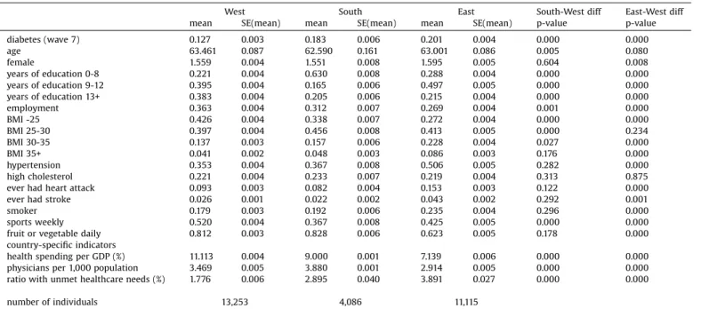
DescriptivestatisticsinTable1showthat,comparedtothe Western European population, Eastern Europeans on average havelesseducation,arelesslikelytobeemployed,haveahigher BMI (particularlyin theobese and severelyobeserange), are moreoftendiagnosedwithhypertension,aremorelikelytohave everhadaheartattackorstroke,smokemoreoften;butplay sportsatleastweeklyoreatfruitorvegetabledailyinasmaller proportion. Southern Europeans haveless education, are less likelyto be employed, havea higher BMI (in the overweight range)andlessoftenplaysportsthanWesternEuropeans,but otherwise the differences are smaller than in the East-West dimension.

Table1

DescriptivestatisticsofthevariablesusedinTable2.

West South East South-Westdiff East-Westdiff

mean SE(mean) mean SE(mean) mean SE(mean) p-value p-value

diabetes(wave7) 0.127 0.003 0.183 0.006 0.201 0.004 0.000 0.000

age 63.461 0.087 62.590 0.161 63.001 0.086 0.005 0.080

female 1.559 0.004 1.551 0.008 1.595 0.005 0.604 0.008

yearsofeducation0-8 0.221 0.004 0.630 0.008 0.288 0.004 0.000 0.000

yearsofeducation9-12 0.395 0.004 0.165 0.006 0.497 0.005 0.000 0.000

yearsofeducation13+ 0.383 0.004 0.205 0.006 0.215 0.004 0.000 0.000

employment 0.363 0.004 0.312 0.007 0.269 0.004 0.001 0.000

BMI-25 0.426 0.004 0.338 0.007 0.272 0.004 0.000 0.000

BMI25-30 0.397 0.004 0.456 0.008 0.413 0.005 0.000 0.234

BMI30-35 0.137 0.003 0.157 0.006 0.228 0.004 0.027 0.000

BMI35+ 0.041 0.002 0.048 0.003 0.086 0.003 0.176 0.000

hypertension 0.353 0.004 0.367 0.008 0.506 0.005 0.282 0.000

highcholesterol 0.221 0.004 0.233 0.007 0.219 0.004 0.313 0.875

everhadheartattack 0.093 0.003 0.082 0.004 0.153 0.003 0.122 0.000

everhadstroke 0.026 0.001 0.022 0.002 0.043 0.002 0.292 0.001

smoker 0.179 0.003 0.192 0.006 0.235 0.004 0.296 0.000

sportsweekly 0.520 0.004 0.367 0.008 0.425 0.005 0.000 0.000

fruitorvegetabledaily 0.812 0.003 0.828 0.006 0.623 0.005 0.178 0.000

country-speciﬁcindicators

healthspendingperGDP(%) 11.113 0.004 9.000 0.001 7.139 0.006 0.000 0.000

physiciansper1,000population 3.469 0.005 3.880 0.001 2.914 0.005 0.000 0.000

ratiowithunmethealthcareneeds(%) 1.776 0.006 2.895 0.040 3.891 0.027 0.000 0.000

numberofindividuals 13,253 4,086 11,115

Apartfromwave7diabetes,allindicatorsaremeasuredinwave4.

Thelasttwocolumnsshowtheresultsoft-testofequalityacrosscountrygroups.

5Seealsothetechnicalreferenceofthepackage(https://github.com/grf-labs/grf/

blob/master/REFERENCE.md),section6.2.ofAtheyetal.(2019)orsection1.3.of AtheyandWager(2019).

6Wetriedvariousotherspeciﬁcationsforthecausalforestsuchasusingthe baselinebuilt-inparametersortuningonlyasubsetoftheparameters,butthe conclusionsdidnotchange.

(5)

Lookingatthecountry-speciﬁcindicators,healthspendingper GDPandthedensityofphysiciansarelower,whiletheprevalence ofunmetneedsishigherintheEastthanintheWest.IntheSouth, these indicators are in between, apart from the number of physicians,whichisthehighestthere.

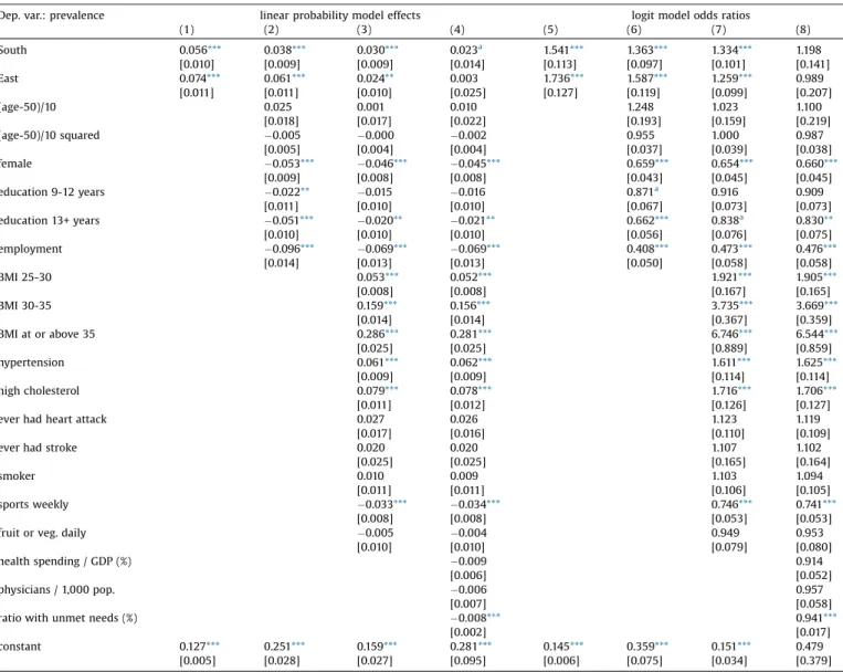
AccordingtoTable2,theunadjustedEast-Westdifferenceof7.4

%points (odds ratio [OR] = 1.74) is only slightly reduced by controlling fordemographic and socio-economicvariables (age, gender,yearsofeducationandemployment)butdecreasestoless than half (to 2.4 %points, OR=1.26) by controlling further for health-related(BMI,hypertension,highcholesterol,heartattack, stroke)andlifestylefactors.TheSouth-Westdifferencedecreases bymorethanone-third,from5.6%pointsto3.0%points(ORfrom 1.54 to1.33) after controlling for these variables. According to Fig.1a,theunadjustedandadjusteddifferencesarefarfromeach otherinSwitzerlandandDenmark,whereasubstantialportionof the better than average prevalence is explained by the more favourabledistributionoftheriskfactors.On theotherhand,in

HungaryandPoland,thebulkoftheworsethanaverageprevalence isexplainedbytheworsevaluesoftheobservedriskfactors.

Ascolumns(4)and(8)inTable2indicate,onceweaddthethree country-speciﬁcindicatorstotheregression(healthspendingper GDP,physicianspercapita,prevalenceofunmetneeds),theEast- WestdifferenceindiabetesprevalencedisappearsandtheSouth- West difference decreases substantially. Thus, differences in healthcareavailabilitylargelyexplaintheresidualdifferencesin prevalence.

4.2.Incidence

Inthefollowing,wefocusonincidence(i.e.onthetransitionto diabetesbetweenwaves4and7)becauseriskfactorsmeasured beforethediagnosis(inwave4)are moreplausiblyexogenous.

Fig.1bandtheﬁrstcolumnofTable3showhowthetransitionrate fromnon-diabetestodiabetesvariesacrosscountriesandregions.

IncidenceissigniﬁcantlyhigherthanaverageinHungary,Spain, Table2

OLSandlogitmodelsofdiabetesprevalenceinSHAREwave7.

Dep.var.:prevalence linearprobabilitymodeleffects logitmodeloddsratios

(1) (2) (3) (4) (5) (6) (7) (8)

South 0.056*** 0.038*** 0.030*** 0.023^a 1.541*** 1.363*** 1.334*** 1.198

[0.010] [0.009] [0.009] [0.014] [0.113] [0.097] [0.101] [0.141]

East 0.074*** 0.061*** 0.024** 0.003 1.736*** 1.587*** 1.259*** 0.989

[0.011] [0.011] [0.010] [0.025] [0.127] [0.119] [0.099] [0.207]

(age-50)/10 0.025 0.001 0.010 1.248 1.023 1.100

[0.018] [0.017] [0.022] [0.193] [0.159] [0.219]

(age-50)/10squared 0.005 0.000 0.002 0.955 1.000 0.987

[0.005] [0.004] [0.004] [0.037] [0.039] [0.038]

female 0.053*** 0.046*** 0.045*** 0.659*** 0.654*** 0.660***

[0.009] [0.008] [0.008] [0.043] [0.045] [0.045]

education9-12years 0.022** 0.015 0.016 0.871^a 0.916 0.909

[0.011] [0.010] [0.010] [0.067] [0.073] [0.073]

education13+years 0.051*** 0.020** 0.021** 0.662*** 0.838^a 0.830**

[0.010] [0.010] [0.010] [0.056] [0.076] [0.075]

employment 0.096*** 0.069*** 0.069*** 0.408*** 0.473*** 0.476***

[0.014] [0.013] [0.013] [0.050] [0.058] [0.058]

BMI25-30 0.053*** 0.052*** 1.921*** 1.905***

[0.008] [0.008] [0.167] [0.165]

BMI30-35 0.159*** 0.156*** 3.735*** 3.669***

[0.014] [0.014] [0.367] [0.359]

BMIatorabove35 0.286*** 0.281*** 6.746*** 6.544***

[0.025] [0.025] [0.889] [0.859]

hypertension 0.061*** 0.062*** 1.611*** 1.625***

[0.009] [0.009] [0.114] [0.114]

highcholesterol 0.079*** 0.078*** 1.716*** 1.706***

[0.011] [0.012] [0.126] [0.127]

everhadheartattack 0.027 0.026 1.123 1.119

[0.017] [0.016] [0.110] [0.109]

everhadstroke 0.020 0.020 1.107 1.102

[0.025] [0.025] [0.165] [0.164]

smoker 0.010 0.009 1.103 1.094

[0.011] [0.011] [0.106] [0.105]

sportsweekly 0.033*** 0.034*** 0.746*** 0.741***

[0.008] [0.008] [0.053] [0.053]

fruitorveg.daily 0.005 0.004 0.949 0.953

[0.010] [0.010] [0.079] [0.080]

healthspending/GDP(%) 0.009 0.914

[0.006] [0.052]

physicians/1,000pop. 0.006 0.957

[0.007] [0.058]

ratiowithunmetneeds(%) 0.008*** 0.941***

[0.002] [0.017]

constant 0.127*** 0.251*** 0.159*** 0.281*** 0.145*** 0.359*** 0.151*** 0.479

[0.005] [0.028] [0.027] [0.095] [0.006] [0.075] [0.034] [0.379]

Numberofobservations:28,454.Allexplanatoryvariablesaremeasuredinwave4.

Standarderrorsinbrackets(OLS:robust),

*** p<0.01.

**p<0.05.

ap<0.1.

(6)

Poland,theCzechRepublic,andlowerinDenmark,Switzerland, France,Germany,SwedenandAustria.Six-yearincidenceisby5.9

%points(OR=2.64)higherinEasternandby4.3%points(OR=2.20) higher in Southern Europe than in Western Europe (4.0%).

AccordingtoTable3,controllingfortheindividual-levelvariables measured atwave 4 reducestheEast-West differenceto3.9 % points(OR=2.01)andtheSouth-Westdifferenceto3.2%points(OR

=1.85).

Among the control variables, the three additional health- related componentsofthemetabolicsyndrome allincreasethe rate of transition to overt diabetes. Even overweight (25BMI<30), which characterises morethan 40% of the 50+

population, isa significantriskfactor(OR =2.1),whilethetwo classesofobesityhaveamarkedlylargereffect(OR=4.0and5.5, notsignificantlydifferentfromeachother).Previoushypertension andhighbloodcholesterolhaveORsaround1.3.Femalegenderand employment are associated with strongly reduced diabetes incidence,whilemeasuredlifestylefactorshaveonlymarginally significanteffects.

Just as in the case of diabetes prevalence, the bulk of the remainingEast-WestdifferenceandalargeportionoftheSouth- Westdifference in diabetesincidenceis explainedbythethree country-speciﬁc healthcare indicators (columns (4) and (8) of Table3).

4.3.Heterogeneityinincidence

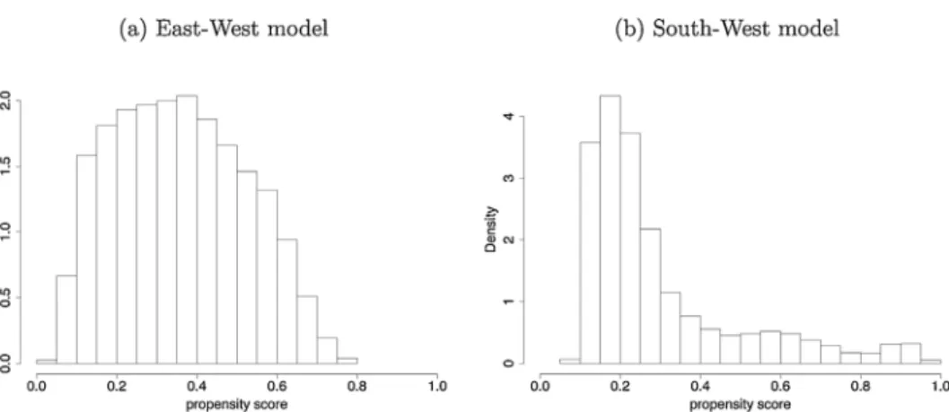
Thedescriptive plots of Fig.2 showthat hypertension,high blood cholesterol and high BMI are associated with a higher probabilityofnewdiabetesdiagnosisinallthreeregions,butto varyingdegrees.Forinstance,theassociationofhypertensionand highcholesterolwiththediagnosisseemstobemorepronounced inEasternEuropethanelsewhere.

Toanalysetheheterogeneityofregionaleffects,wetraincausal forestsasexplainedinsection3.2,usingthesameindividual-level controlvariablesasincolumn(3) ofTable3.Thecausalforests yield very similar estimates for the average adjusted regional differences in diabetes incidence as the controlled linear Table3

OLSandlogitmodelsofnewdiabetesdiagnosisbetweenSHAREwaves4and7.

Dep.var.:incidence linearprobabilitymodeleffects logitmodeloddsratios

(1) (2) (3) (4) (5) (6) (7) (8)

South 0.043*** 0.035*** 0.032*** 0.022** 2.195*** 1.953*** 1.847*** 1.391^a

[0.007] [0.007] [0.007] [0.010] [0.245] [0.215] [0.210] [0.248]

East 0.059*** 0.055*** 0.039*** 0.010 2.642*** 2.513*** 2.009*** 1.036

[0.009] [0.009] [0.009] [0.020] [0.319] [0.303] [0.244] [0.346]

(age-50)/10 0.012 0.018 0.023 0.819 0.716 0.655

[0.014] [0.014] [0.017] [0.187] [0.167] [0.192]

(age-50)/10squared 0.005 0.007â 0.006â 1.080 1.123** 1.114â

[0.003] [0.003] [0.003] [0.059] [0.064] [0.062]

female 0.032*** 0.027*** 0.027*** 0.574*** 0.601*** 0.605***

[0.006] [0.006] [0.006] [0.059] [0.063] [0.063]

education9-12years 0.012 0.009 0.009 0.855 0.891 0.886

[0.008] [0.008] [0.008] [0.107] [0.114] [0.113]

education13+years 0.020** 0.008 0.009 0.713** 0.858 0.857

[0.008] [0.008] [0.008] [0.101] [0.126] [0.126]

employment 0.034*** 0.027** 0.027** 0.507*** 0.541*** 0.542***

[0.011] [0.011] [0.011] [0.101] [0.109] [0.108]

BMI25-30 0.026*** 0.026*** 2.068*** 2.038***

[0.005] [0.005] [0.269] [0.266]

BMI30-35 0.082*** 0.081*** 4.005*** 3.948***

[0.012] [0.012] [0.606] [0.595]

BMIatorabove35 0.118*** 0.116*** 5.462*** 5.306***

[0.023] [0.023] [1.135] [1.105]

hypertension 0.015** 0.016** 1.301** 1.326***

[0.007] [0.007] [0.138] [0.140]

highcholesterol 0.017â 0.015â 1.300** 1.261â

[0.009] [0.009] [0.156] [0.154]

everhadheartattack 0.009 0.009 0.878 0.879

[0.010] [0.010] [0.117] [0.117]

everhadstroke 0.037â 0.036 1.473â 1.454â

[0.022] [0.022] [0.323] [0.319]

smoker 0.009 0.009 1.182 1.178

[0.008] [0.008] [0.176] [0.176]

sportsweekly 0.007 0.007 0.860 0.860

[0.006] [0.006] [0.095] [0.096]

fruitorveg.daily 0.009 0.008 0.857 0.865

[0.008] [0.008] [0.104] [0.106]

healthspending/GDP(%) 0.009^a 0.822**

[0.005] [0.074]

physicians/1,000pop. 0.009 0.895

[0.005] [0.083]

ratiowithunmetneeds(%) 0.005*** 0.923***

[0.002] [0.024]

constant 0.040*** 0.117*** 0.082*** 0.233*** 0.041*** 0.149*** 0.070*** 1.237

[0.003] [0.022] [0.022] [0.076] [0.003] [0.049] [0.025] [1.549]

Numberofobservations:24,967.Allexplanatoryvariablesaremeasuredinwave4.

Standarderrorsinbrackets(OLS:robust),

*** p<0.01.

**p<0.05.

ap<0.1.

(7)

probabilitymodelinTable3:3.8%points(S.E.=0.6%point)forthe East-West difference and 3.9 %points (S.E.=0.4 %point) for the South-West difference.However, thevalueadded of thecausal forestapproachisthatitautomaticallyyieldseffectestimatesfor each individual,sothattheycanbeaggregatedbydifferentrisk factors.

Thesubsample-specificadjustedregionaldifferences(calculat- edfromequation(4)inAppendixA),their95%confidenceintervals andthestatisticalsignificanceofthebetween-groupvariationsare displayed in Fig. 3.⁷ The adjusted East-West difference is significantly higher for individuals with lower education level, withoutemploymentinwave4,withhigherBMI,withprevious hypertension or high cholesterol, in such a way that the least vulnerable groups have essentially noexcess transition risk to diabetesintheEastcomparedtotheWest.Forinstance,theeffect estimateis1.1%point(notsignificantlydifferentfromzeroatthe 10%level)forthosewithmorethan12yearsofschoolingbut5.5% points for those with at most 8 years, or 1.3 %points (not significantlydifferentfromzeroatthe5%level)forthosewithout

hypertensionand7.0 %pointsfor thosewithit. Amonglifestyle factors,smokingincreasestheexcessrisksigniﬁcantlyatthe5%

level. Meanwhile, effect heterogeneity is not signiﬁcant across gender,age,previousheartattackorweeklysportsactivity.

Compared tothethe East-Westdimension, heterogeneityis much less pronounced in theSouth-West dimension (Fig. 3b), wheretheeffectestimateisstatisticallysigniﬁcantlypositivein eachsubsample.Signiﬁcantheterogeneityisobservedonlybylevel ofeducation,previousemploymentstatus,BMIandsportsactivity.

Forrobustness check, AppendixBdisplays subsample-specific regional effects that were estimated by OLS regressions run on different subsamples, using the same control variables as in column (3) ofTable3.(Forillustration,thesubsamplesweredefinedbyhealth status.)TheOLSpointestimatesaresimilartothecausalforestones buthavelargerstandarderrors becausethecausalforestmethodology automaticallychoosestheheterogeneitiesthatshouldbeincludedin themodel(whilethesubsample-specificOLSmodelsimplicitlyuse manyinteractiontermsbetweenthecontrolvariables).

Appendix C contains the goodness-of-ﬁt analysis of the estimated causal forests. According to Fig. C1, the propensity scores are mainly between 0.05 and 0.95, hence the overlap assumption holds both for the East-West and the South-West model.TableC1showsthatthelarge(standardized)differencesin the explanatory variables (especially in BMI, hypertension and Fig.2.TransitionprobabilitiestodiabetesbetweenSHAREwaves4and7,byhypertension,highcholesterolandBMIcategorymeasuredinwave4.

7Theﬁguresdonotshowheterogeneitiesbythepresenceorabsenceofprevious strokebecausetheratioofindividualswhoeverhadastrokeisonly2-4%hencethe regionaleffectsforthemareveryimpreciselyestimated.

(8)

Fig.3. Averageindividual-leveladjustedregionaldifferencesbyvariousriskfactors,with95%conﬁdenceintervalsandwiththestatisticalsigniﬁcanceofthebetween-group variation(***p<0.01,**p<0.05,*p<0.1,n.sp0.1).

Table4

ModelsoftheprobabilityofreportingweightlossduetodietinSHAREwave7.

linearprobabilitymodeleffects logitmodeloddsratios

(1) (2) (3) (4)

South 0.007 0.025*** 0.894 0.650**

[0.012] [0.010] [0.175] [0.112]

East 0.051*** 0.054*** 0.277*** 0.268***

[0.007] [0.007] [0.046] [0.046]

Westdiabetesinwave7 0.077** 0.101** 2.245*** 2.826***

[0.035] [0.040] [0.644] [0.849]

Southdiabetesinwave7 0.007 0.022 1.109 1.463

[0.025] [0.026] [0.429] [0.641]

Eastdiabetesinwave7 0.038^a 0.035^a 2.886*** 2.717**

[0.019] [0.021] [1.069] [1.098]

(age-50)/10 0.005 1.274

[0.021] [0.503]

(age-50)/10squared 0.005 0.880

[0.004] [0.081]

female 0.021** 1.456**

[0.009] [0.217]

education9-12years 0.012 0.800

[0.010] [0.149]

education13+years 0.006 1.101

[0.010] [0.186]

employment 0.009 0.861

[0.011] [0.153]

constant 0.072*** 0.062** 0.078*** 0.056***

[0.006] [0.028] [0.007] [0.027]

Sample:non-diabeticandoverweightorobeseinwave4.Numberofobservations:10,406.

Theexplanatoryvariablesaremeasuredinwave4,apartfromdiabetesinwave7.

Standarderrorsinbrackets(OLS:robust).

*** p<0.01.

**p<0.05.

ap<0.1.

(9)

dailyfruitorvegetableconsumptionintheEast-Westdimension;

andBMI,educationandweeklysportsactivityintheSouth-West dimension) are substantially reduced after weighting with the inverseofthepropensityscore,whichpointstoareasonablepost- estimation balanceacrosstheexplanatory variables. Infact, for most variables, the absolute value of the inverse-propensity weightedstandardizeddifferenceisbelow0.10,thethresholdof appropriatebalanceassuggestedbyAustin(2009).

Finally, Table C2 displays the results of the “best linear prediction” method of Chernozhukov et al. (2018a,b). For the East-Westmodel,neithercoefficientsdiffersignificantlyfromone, suggesting an appropriate fit both in terms of the average treatmenteffectandtreatmenteffectheterogeneity.Meanwhile, fortheSouth-Westmodel,thecoefficientoftheaverageeffectis essentiallyone,butthecoefficientofeffectheterogeneitytakesan imprecisely estimated negative value (which does not differ significantlyeitherfromzeroorone).InlinewithFig.3,thisalso suggestsamorehomogeneoustreatmenteffectintheSouth-West dimension.

4.4.Management

Finally, we analyse how the new diagnosis of diabetes is associatedwithchangesindietaryhabits.Table4 indicatesthat among the overweight or obese population in wave 4 who remainednon-diabeticthroughoutwaves47,weightlossdueto dietinwave7waslessprevalentby5.1%pointsinEasternEurope thaninWesternEurope(OR=0.28),whiletherewasnodifference in theSouth-West dimension.Comparedtothis population,the diagnosisofdiabetesincreasedtheprevalenceofweightlossinthe West(by7.7%points)aswellasintheEast(by3.8%points),while therewasnochangeintheSouth.Theseresultsareonlyslightly affected when control variables are included in the analysis, although then the South-West difference in the prevalence of weight loss in the non-diabetic (baseline) sample becomes statisticallysigniﬁcantlynegative(2.5%pointslowerintheSouth thanintheWest).Hence,inWesternaswellasinEasternEurope,a newdiabetesdiagnosisisassociatedwithasubstantiallyincreased likelihood ofweightloss duetodiet butnosuchassociationis foundintheSouth.

Lookingattwo-yeartransitionstodiabetesandusingdatafrom waves 4to7fortheavailablecountries, weobservethatinthe wavewhendiabetesisﬁrstreported,11.9%oftherespondentswho wereoverweightorobeseinthepreviouswavereportweightloss duetodiet.Thisratioisaround7-8%twoandfouryearsbeforeand twoandfouryearsafterthediagnosis,whichisclosetotheaverage probabilityof weightlossdue todiet amongtheoverweightor obese population (6.7%). Hence, the change in dietary habits mostly coincides with the diagnosis of diabetes and thus the analysisabovemeritsattention.

5.Conclusions

Usingdatafromthreeregionsand15countriesinEurope,we documented that diabetes prevalence and incidence are much higherintheSouthandEastthanintheWest,andonly2570%of these differences disappear by controlling for individual-level demographic and socio-economic characteristics, health status and health behaviour. Thecountry-speciﬁc indicators of health spending,availabilityofphysiciansandprevalenceofunmetneeds explainalargeportionoftheremainingpart.Thus,theobserved regionaldifferencesarelikelytobecausedbyacombinationofthe differences in healthcare systems and in individual socio- economicandhealth-relatedvariables.

HeterogeneityanalysesshowedthattheEast-Westdifferencein incidenceisessentiallyzerofortheleastvulnerablegroupssuchas

thosewithtertiaryeducationorwithouthypertension.Atthesame time,WesternEuropeancountriesfaremuchbetterinpreventing diabetesamonglower-educatedindividualsandamongthosewith comorbidities.Meanwhile,theSouth-Westdifferenceseemsmore stableacrossthesedimensions.

Our results on the association of diabetes prevalence and incidence with regional, socio-economic, health and lifestyle indicatorsarein linewiththeexistingliterature (Agardhet al., 2011;Espeltetal.,2013;IDF,2019;DiabetesPreventionProgram ResearchGroup,2002;Narayanetal.,2007;Whitingetal.,2011).

Ontheotherhand,weextendourunderstandingoftheregional differencesindiabetesbyshowingthatthesedifferencesarelarger amongthehigh-riskindividualsand–atleastforEasternEurope– areessentiallyzeroamongthelowest-riskpopulation.

Usinganindicatorofchangeindietaryhabits,wealsofound thatoverweightorobeseindividualsarelesslikelytochangediet effectivelyintheSouthandespeciallyintheEastthanintheWest.

However, among people newly diagnosed with diabetes, the prevalenceofweightlossduetodietissimilarintheEastandinthe West.Thus,atleastfortheEast,wedonotseeevidencethatthe higher incidence of diabetes would be coupled with worse managementasmeasuredbyweightlossduetodiet.

Theanalysisissubjecttosomelimitations.First,itusesself- reported data on diagnosed diabetes, although undiagnosed cases make up one-third to one-half of total (diagnosed and undiagnosed)prevalence(IDF,2019).Theexplanatoryvariables such as BMI, hypertension or high blood cholesterol are also self-reported and thus are subject to measurement error.

Second, the three examined regions are not homogeneous, hence, by construction, any regional analysis overlooks the differences acrosscountries within a region. (Meanwhile,the country-level sample sizes are generally too small to yield powerful conclusions.) Third, diabetes incidence is only analysed over a six-year horizon, due to the changing country-compositionoftheSHAREsample.Finally,onlyacrude and self-reported measureof diabetesmanagement – weight lossduetodiet– isusedbecausewedonotobservedetailed outpatient,inpatientorlaboratorytestingdata(apartfromthe rawnumberofdoctoralvisits).

Inthe6thwaveofSHARE,bloodsampleswerecollectedfrom around 24 thousand individuals from 12 countries. Since the blood parameters (including glycated hemoglobin [HbA1c]

measurements)arenotyetavailableforresearchers,it remains for future research to analyse the prevalence of undiagnosed diabetesandthequalityofdiabetesmanagementbasedonblood sampleresults.

Overall, we found that diabetes incidence in Eastern and Southern Europeis more than twofold higher thanin Western Europe,andthesedifferencescannotbeexplainedbydifferencesin the demographic composition, education level and economic activityofthepopulation.Ourresultssuggestthattoreducethe regional differences in diabetes incidence in Europe, more emphasis should be put on the prevention of diabetes among individuals moreprone tothediseasein Easternand Southern Europe,whichcouldatleastpartlybeachievedbyinterventions aimed at preventing obesity, hypertension or high cholesterol amongthehigh-riskpopulation.

Funding

Theauthorsweresupportedbythe“Lendület”programmeof the Hungarian Academy of Sciences (grant number: LP2018-2/

2018). Péter Elek was supported by the János Bolyai Research Scholarship of the Hungarian Academy of Sciences and by the ÚNKP-19-4NewNationalExcellenceProgrammeoftheHungarian MinistryforInnovationandTechnology.