DOI:10.28974/idojaras.2018.2.6
IDŐJÁRÁS
Quarterly Journal of the Hungarian Meteorological Service Vol. 122, No. 2, April – June, 2018, pp. 203–216
Parametric or non-parametric: analysis of rainfall time series at a Hungarian meteorological station
Tímea Kocsis1*and Angéla Anda2
1 Budapest Business School College of Commerce, Catering and Tourism Department of Methodology,
Alkotmány Str. 9-11, H-1054 Budapest, Hungary
2 University of Pannonia Georgikon
Faculty Department of Meteorology and Water Management, Festetics Str. 7. H-8360 Keszthely,Hungary
*Corresponding author E-mail: JakuschneKocsis.Timea@uni-bge.hu
(Manuscript received in final form February 2, 2017)
Abstract⎯ Parametric methods (linear trend, t-test for slope) for analyzing time series are the simplest methods to get insight to the changes in a variable over time. These methods have a requirement for normal distribution of the population that can be a limit for application. Non-parametric methods are distribution-free methods, and investigators can have a more sophisticated view to the variable tendencies in time series. 144-year-long time series of precipitation data measured at the meteorological station in Keszthely, Hungary (latitude: 46°44′, longitude: 17°14′, elevation: 124 m above Baltic sea level) were analyzed by Mann-Kendall trend test for detecting tendencies in the time series. Sen’s slope estimator was applied to estimate the slope of the linear changes. In average, 44 mm decline can be shown for 100 years in the annual sum, 29.7 mm and 25.7 mm in the precipitation sum of spring and autumn (in 100 years), respectively. The rainfall sum of winter increased by 15.4 mm. Sums of April, May, and October declined by 10.8 mm, 13 mm, and 20.9 mm, respectively, according to one-tailed Mann-Kendall tests. These results were compared to the previous results of the authors carried out by parametric methods. Results of two-tailed tests of parametric and non-parametric methods are easily comparable. Parametric method (linear trend) proved significant decreasing tendencies for spring, April, and October. Non- parametric Mann-Kendall tests show significant declining tendencies for spring, autumn, and October.
Key-words: Kendall’s tau, Mann-Kendall trend test, Sen’s slope estimator, precipitation changes, Keszthely, Hungary
1. Introduction
Climate change is one of the problems that mankind should face in the 21st century.
According to the last IPCC report (2013), human role in the process has no doubt (95% is the probability that human influence has been dominant on the present changes of climate system). Climate change will probably affect all parts of the Earth, and in the center of Europe, the Carpathian Region will be influenced as well. In some cases, the volume and direction of the changes in climate model simulations are uncertain. Hydrological cycle is an element of the climate system that is expected to change, and the signs of these amendments can already be detected. Precipitation in average over mid-latitude land areas of the Northern Hemisphere has increased from 1901 (medium confidence) according to IPCC AR5 (2013). Heavy precipitation events and increase in intensity and frequency of rainfall are very likely (90% probability) over mid-latitude land masses (IPCC, 2013). Precipitation strongly influences the water cycle from local to global scales. Any modification in the amount or distribution of rainfall has significant impact on the water availability, and therefore, water management. Hungary, which occupies the middle of the Carpathian-Basin, has long-experienced significant temporal and spatial variations in precipitation. In recent decades, due to the hardships faced by the state complying with decreasing rainfall amount, studies related to precipitation events are extremely beneficial.
The prediction of the effects of climate change on the Carpathian Region (including Hungary) requires regional climate scenarios with adequate temporal and spatial resolution, capable of translating global phenomena to a local scale. Bartholy et al. (2004) applied regional models to estimate the regional effects of climate change in the Balaton Lake–Sió Canal catchment area, using ECHAM/GCM outputs. This catchment area (which also includes Keszthely meteorological station) is one of the most vulnerable regions in Hungary because of its economical and touristic importance and unique treasure of nature. According to Bartholy et al.
(2005), the amount of precipitation will decline by 25–35% in the summer half-year and by 0–10% in the winter half-year on the Balaton Lake–Sió Canal catchment area. The regional model runs for the Carpathian Basin (RCMs) using the A2 and B2 global emission scenarios of the IPCC AR4 (2007), expect more than 2.5 and less than 4.8 °C temperature rise for all seasons and both scenarios (Bartholy et al., 2007).
A 20–33% decrease in precipitation is predicted for the summer half-year and there is high uncertainty for the rainfall for the winter half-year (Bartholy et al., 2007). The earlier results of the authors harmonizes with their latest projection carried out in the PRUDENCE European Project’s model application (Bartholy et al., 2009). These statements were enhanced by Bartholy et al. (2008) and by the Hungarian Meteorological Service (OMSZ, 2010) according to further regional climate model simulations. Pongrácz et al. (2011) and Kis et al. (2014) communicated similar results for projection of the future climate in Hungary. Pongrácz et al. (2014) project significant increase in drought-related indices in summer by the end of the 21st
century. Bartholy et al. (2015) examined precipitation indices and project that frequency of extreme precipitation will increase in Central Europe, except of summer, when decreasing tendency is very likely. For the tendencies of the past, Szalai et al., (2005) stated that the annual precipitation amount decreased by 11%
between 1901 and 2004, according to the analysis of the Hungarian Meteorological Service. The biggest decline could be experienced in spring; it was 25% for the above mentioned period. Bodri (2004) suggested that slow decrease of precipitation with a noticeable increase in precipitation variability are characteristic for the 20th century.
While the northern and western part of Europe gets more precipitation in parallel with the warming tendency, Hungary, similarly to the region of the Mediterranean Sea, gets less rainfall. The water balance has deficit, since the difference between water income and outflow is increasing. Between 1901 and 2009, the highest precipitation decline over the territory of Hungary occurred in the spring, nearly 20%
(Lakatos and Bihari, 2011). Bartholy and Pongrácz (2005, 2007, 2010) examined several precipitation extreme indices and suggested that regional intensity and frequency of extreme precipitation increased in the Carpathian Basin in the second half of the last century, while the total precipitation decreased.
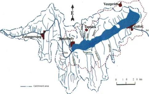
The goal of this study is to analyze the long-term data series of the meteorological measurements of precipitation amount at the meteorological station at Keszthely, Trans-Danubia, Hungary (N 46°44’, E 17°14’, Fig. 1) from the point of view of climate and statistics. Our aim is to analyze the dataset by non-parametric methods and compare the results to our previous findings derived from parametric time series analyses. A non-parametric method, the Mann-Kendall trend test, that was applied in this research, is widespread for analyzing meteorological (such as precipitation sums) and hydrological data. The Sen’s slope estimator was applied as non-parametric method for determining the slope of the tendencies.
Fig. 1. Catchment area of the Balaton Lake.
(source: website of the Hungarian Water Inspectorate)
Several examples can be found in the literature for application of the Mann- Kendall trend test, e.g., Patle and Libang (2014) argued on trend analysis of annual and seasonal rainfall the northeastern region of India, Salmi et al. (2002) analyzed the trends of atmospheric pollutants in Finnland. Meteorological applications can be read in Rahman and Begum (2013), who determined trends of rainfall of the largest island in Bangladesh. Ganguly et al. (2015) investigated the tendencies of rainfall in Himachal Pradesh (state in North India) between 1950 and 2005. Gavrilov et al. (2015a, 2015b, 2016) examined trends of air temperature by Mann-Kendall test in Vojvodina, Serbia. Salami et al. (2014) applied this non- parametric trend test for the analysis of hydro-meteorological variables in Nigeria.
Mapurisa and Chikodzi (2014) made an assessment of trends of monthly and seasonal rainfall in Southeast Zimbabwe. Karmeshu (2012) investigated the temperature- and precipitation changes in the northeastern part of United States.
Hydrological utilization is given by Hamed (2008). Burn and Hag Elnur (2002) estimated the trends and variability of 18 hydrological variables by Mann-Kendall trend test. Hirsch et al. (1991) used the method for investigation of stream water quality.
2. Data and methods
Monthly amounts of precipitation were analyzed from 1871 to 2014 measured at the beginning in the territory of the ancient Georgikon Academy of Agriculture at Keszthely, then at the meteorological station of the Hungarian Meteorological Service. The dataset was provided by the Department of Meteorology and Water Management of University of Pannonia Georgikon Faculty (Keszthely). This dataset is special, because few stations in Hungary have continuous measurements of more than 140 years with detailed historical background (Kocsis and Anda, 2006). The dataset was analyzed in three sessions: annual amounts, seasonal amounts and monthly precipitation sums. Seasons of temperate climate were performed as common in meteorology, e.g., spring: March, April, May, etc.
2.1. The Mann-Kendall trend test
Mann-Kendall trend test is widespread in climatological and hydrological time series analysis, because it is simple and robust, it can cope with missing values and values under detection limit (Gavrilov et al., 2016). This non-parametric test is commonly used to detect monotonic tendencies in series of environmental data, too (Pohlert, 2016). This method has no requirement for the distribution of the population, as the regression method has a requirement for normal distribution.
No assumption of the normality is required (Helsel and Hirsh, 2002). Hirsch et al. (1982) and Hirsch and Slack (1984) developed the method and introduced seasonal Mann-Kendall test for data that are serially dependent. Hamed and Rao
(1998) developed a modified Mann-Kendall test for autocorrelated data. Yue et al.
(2002) investigated the power of the Mann-Kendall test in hydrological series.
The Mann-Kendall trend test is based upon the work of Mann (1945) and Kendall (1975), and is closely related to the Kendall’s rank correlation coefficient.
The methodology is introduced following the detailed descriptions given by Gilbert (1987) and Hipel and McLeod (1994) as follows:
In case of determining the presence of monotonic trend in a time series, the null hypothesis (H0) of the Mann-Kendall test is that the data come from a population where random variables are independent and identically distributed.
The alternative hypothesis (Ha) is that the data follow a monotonic trend over time. The Mann-Kendall test statistic is given as
= ∑ ∑ ( − ), (1)
where j>k, and
( ) = +1, > 0 0, = 0
−1, < 0. (2)
Kendall (1975) proved that S is asymptotically normally distributed with the following parameters (mean and variance):
= 0
= ( − 1)(2 + 5) − ∑ ( − 1)(2 + 5) /18, (3) where p is the number of the tied groups in the data set, tj is the number of data
in the jth tied group, and n is the number of data in the time series.
Positive value of S means that there is an increasing trend, negative value of S means the opposite, there is a decreasing trend with time. It was proven that if the number of data is above 10, the standard normal variate Z can be used for hypothesis test:
=
( ) / , > 0 0, = 0
( ) / , < 0
. (4)
During the hypothesis test, α=5% significance level was used in the two- tailed and one-tailed tests as well, and statistical significance was determined. S is closely related to the Kendall’s rank correlation coefficient (τ):
=
, (5)where D is the possible number of data pairs from n members of the dataset:
= . (6)
After detecting the non-parametric trend, the Sen’s slope estimator was applied. This is a non-parametric method that can calculate the change per time unit (direction and volume). Detailed description of the method is given by Sen (1968). Not only the value of the slope, but also the confidence interval was estimated under 1–α=95% probability level.
SPSS 17.0 and Addinsoft’s XLSTAT (2016) was used for carrying out the computations.
3. Results
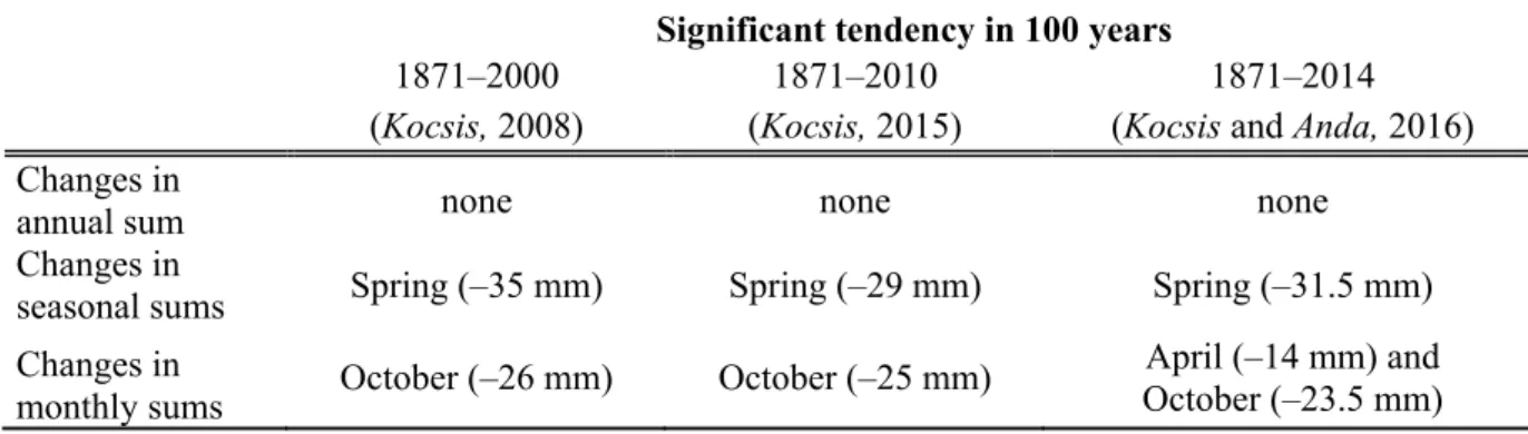
Our previous studies focused on linear trend approximation for analyzing the long-time series of precipitation measured at Keszthely station (Hungary) (Kocsis, 2008; Kocsis and Anda, 2016). Results are summarized in Table 1. It can be stated that statistically significant changes could be detected by linear regression method with parametric test for the slope by two-tailed t-test for spring, and among the monthly data of April and October. Table 2 presents that the requirements for the normal distribution for the population are fulfilled, tested by the Kolmogorov- Smirnov test for distribution. However, in some cases (February, March, July, and November), the distribution cannot be accepted as normal distribution according to p-value (α=5%). For this reason, non-parametric methods were used to analyze all the data set (annual sums, seasonal and monthly sums).
Table 1. Summary of the previous findings using linear trend and two tailed t-test for testing the significance of the slope
Significant tendency in 100 years
1871–2000 1871–2010 1871–2014
(Kocsis, 2008) (Kocsis, 2015) (Kocsis and Anda, 2016) Changes in
annual sum none none none
Changes in
seasonal sums Spring (–35 mm) Spring (–29 mm) Spring (–31.5 mm) Changes in
monthly sums October (–26 mm) October (–25 mm) April (–14 mm) and October (–23.5 mm)
Table 2. Results of the test of normal distribution
Distribution (Kolmogorov-Smirnov test) H0: The sample follows a normal distribution Ha: The sample does not follow a normal distribution
Hypothesis accepted at α=5% p-value
Annual sum H0 35.2%
Spring H0 42.1%
Summer H0 80.0%
Autumn H0 53.1%
Winter H0 91.0%
January H0 34.7%
February Ha 4.7%
March Ha 3.6%
April H0 5.3%
May H0 28.6%
June H0 75.2%
July Ha 2.5%
August H0 25.6%
September H0 47.4%
October H0 5.7%
November Ha 3.1%
December H0 7.1%
As the first step, the Kendall’s tau rank correlation coefficient was determined to show the sign of the relationship between time and the variables.
Tau was first tested by the two-tailed test (Table 3). Significance level was stated at α=5%. In two-tailed tests, p-values proved significant negative relationships for spring, autumn, and among the monthly sums, for October.
P-values of some other monthly sums were near to the limit, so one-tailed tests according to the sign of Kendall’s tau were also used. P-values in one-tailed tests show the presence of negative relationship in the annual sum, precipitation sums in spring, autumn, April, May, and October, and positive relationship for the winter (Table 3).
Table 3. Values of Kendall’s rank correlation coefficient and their significance
Kendall τ
Two-tailed test (τ≠0) One-tailed test (τ<0 or τ>0)
p-value p-value
*significant at α=5%
Annual sum –0.096 8.9% 4.5%*
Spring –0.159 0.5%* 0.2%*
Summer –0.036 51.9% 26.0%
Autumn –0.112 4.6%* 2.3%*
Winter 0.096 8.8% 4.4%*
January 0.042 45.2% 22.6%
February 0.063 26.1% 13.0%
March –0.054 33.9% 16.9%
April –0.107 5.7% 2.8%*
May –0.104 6.4% 3.2%
June 0.01 86.3% 43.1%
July –0.018 74.4% 37.2%
August –0.042 45.3% 22.7%
September –0.054 33.4% 16.7%
October –0.153 0.7%* 0.3%*
November 0.012 83.4% 41.7%
December 0.061 27.7% 13.9%
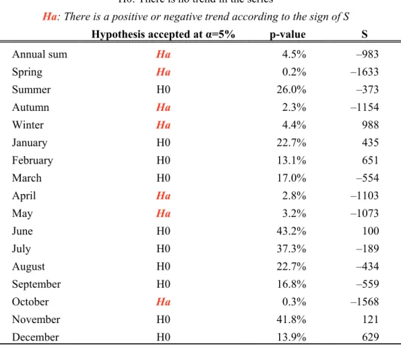
Based on the Kendall’s tau (τ), the Mann-Kendall trend test was used to detect monotonic trends in the time series. First two-tailed (Table 4) and then one- tailed z-tests were applied according to the sign of the calculated S value, respectively (Table 5). Decision about the statistical significance was made using
empirical significance level (p-value) compared to α=5%. The two-tailed Mann- Kendall test (with the alternative hypothesis that there is no trend in the time series) gave significant result for spring, autumn, and October in concordance with the results for the tests for τ. Seasonally in spring and autumn, while among the months, in October the presence of significant monotonic trend could be found. One-tailed tests have an alternative hypothesis, that in the time series, a negative/positive trend is present according to the sign of computed S statistics, respectively. These tests gave the results in accordance to the one-tailed tests for τ, as S and τ statistics are related. According to p-values, significant declining trend can be experienced in the annual sum, precipitation sums in spring, autumn, April, May, and October, and increasing trend can be shown for the winter.
Table 4. Results of the two-tailed Mann-Kendall trend test
Mann–Kendall trend test (two-tailed) H0: There is no trend in the series
Ha: There is a trend in the series
Hypothesis accepted at α=5% p-value
Annual sum H0 9.0%
Spring Ha 0.5%
Summer H0 52.1%
Autumn Ha 4.6%
Winter H0 8.8%
January H0 45.3%
February H0 26.1%
March H0 33.9%
April H0 5.7%
May H0 6.4%
June H0 86.4%
July H0 74.5%
August H0 45.4%
September H0 33.5%
October Ha 0.7%
November H0 83.6%
December H0 27.8%
Table 5. Results of the one-tailed Mann-Kendall trend test
Mann-Kendall trend test (one-tailed) H0: There is no trend in the series
Ha: There is a positive or negative trend according to the sign of S
Hypothesis accepted at α=5% p-value S
Annual sum Ha 4.5% –983
Spring Ha 0.2% –1633
Summer H0 26.0% –373
Autumn Ha 2.3% –1154
Winter Ha 4.4% 988
January H0 22.7% 435
February H0 13.1% 651
March H0 17.0% –554
April Ha 2.8% –1103
May Ha 3.2% –1073
June H0 43.2% 100
July H0 37.3% –189
August H0 22.7% –434
September H0 16.8% –559
October Ha 0.3% –1568
November H0 41.8% 121
December H0 13.9% 629
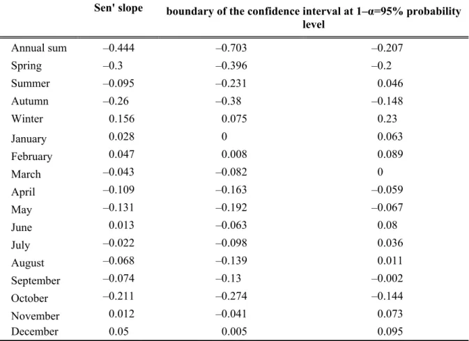
The Sen’s slope estimator was used to determine the slope of the trend (linear change per time unit). Confidence interval is also given for the slope. This interval contains the real value of the slope of the tendency in the population by the probability of 95% (Table 6). According to the one-tailed Mann-Kendall test, the decreasing tendencies are the follows for 100 years on average: the annual sum decreased by 44 mm, the precipitation sum of spring and autumn declined by 29.7 mm and 25.7 mm, respectively. The rainfall sum of winter increased by 15.4 mm.
Sums of April, May, and October declined by 10.8 mm, 13 mm, and 20.9 mm, respectively.
Table 6. Values of the Sen’s slope and their confidence interval
Sen' slope
Lower Upper boundary of the confidence interval at 1–α=95% probability
level
Annual sum –0.444 –0.703 –0.207
Spring –0.3 –0.396 –0.2
Summer –0.095 –0.231 0.046
Autumn –0.26 –0.38 –0.148
Winter 0.156 0.075 0.23
January 0.028 0 0.063
February 0.047 0.008 0.089
March –0.043 –0.082 0
April –0.109 –0.163 –0.059
May –0.131 –0.192 –0.067
June 0.013 –0.063 0.08
July –0.022 –0.098 0.036
August –0.068 –0.139 0.011
September –0.074 –0.13 –0.002
October –0.211 –0.274 –0.144
November 0.012 –0.041 0.073
December 0.05 0.005 0.095
4. Discussion
Parametric methods (linear trend, t-test for slope) for analyzing time series are the simplest methods to get insight to the changes of a variable over time. These methods have a requirement for normal distribution of the population that can be a limit for application. Non-parametric methods are distribution-free methods, and researchers can have a more sophisticated view to the changing tendencies. Our previous results can be accepted, but the Mann-Kendall trend test proved other signs of precipitation changes at the examined meteorological station. One-tailed Mann-Kendall trend tests gave the evidence that decreasing tendencies can be statistically proven in the annual sum by 44 mm for 100 years on average, in the precipitation sum of spring and autumn by 29.7 mm and 25.7 mm, respectively.
The rainfall sum of winter increased by 15.4 mm. Sums of April, May, and
October declined by 10.8 mm, 13 mm, and 20.9 mm, respectively. These results are parallel to the literature in the direction of the precipitation changes, but are not clearly in accordance regarding the volume of the changes estimated for the region of the examined meteorological station (Keszthely, Trans-Danubia, Hungary). Results of two-tailed tests of previous parametric and recent non- parametric methods are easily comparable. Parametric method (linear trend) proved significant tendencies for spring, April, and October (deceasing tendencies). Two-tailed non-parametric Mann-Kendall trend tests show significant tendencies for spring, autumn, and October (declining trends).
Advantage of the non-parametric methods, that is fewer requirements for application, and the results derived from this research are more consistent with the literature. Declining tendencies of precipitation sums in spring and autumn possibly have unfavorable effect on the water-budget of the soil and Balaton Lake.
References
Barhtoly, J. and Pongrácz, R. 2005: Extremes of ground-based and satellite measurements in the vegetation period for the Carpathian Basin. Phys. Chem. Earth 30, 81–89.
https://doi.org/10.1016/j.pce.2004.08.012
Barhtoly, J. and Pongrácz, R. 2007: Regional analysis of extreme temperature and precipitation indices for the Carpathian Basin from 1946 to 2001. Glob. Planet. Change 57, 83–95.
https://doi.org/10.1016/j.gloplacha.2006.11.00
Bartholy, J., Mika, J., Pongrácz, R., and Schlanger, V. 2005: A globális felmelegedés éghajlati sajátosságai a Kárpát-medencében. In (ed.: Takács-Sánta A.) Éghajlatváltozás a világban és Magyarországon. Budapest. 105–139. (in Hungarian)
Bartholy, J. and Pongrácz, R., 2010: Analysis of precipitation conditions for the Carpathian Basin based on extreme indices in the 20th century and climate simulation for 2050 and 2100. Phys. Chem.
Earth 35, 43–51. https://doi.org/10.1016/j.pce.2010.03.011
Bartholy, J., Pongrácz, R., and Gelybó, Gy., 2007: Regional climate change in Hungary for 2071–2100.
Appl. Ecol. Environ. Res. 5, 1–17. https://doi.org/10.15666/aeer/0501_001017
Bartholy, J., Pongrácz, R., Gelybó, Gy., and Szabó, P., 2008. Analysis of expected climate change in the Carpathian Basin using the PRUDENCE results. Időjárás 112, 249–264.
Bartholy, J., Pongrácz, R., Gelybó, Gy., and Szabó, P. 2009: Analysis of expected climate change in the Carpathian Basin using the PRUDENCE results. Időjárás Special Issue 112 (3-4): 249-265 Bartholy, J., Pongrácz, R., and Kis, A. 2015: Projected changes of extreme precipitation using multi-
model approach. Időjárás 119. 129–142.
Bartholy, J., Pongrácz, R., Matyasovszky, I., and Schlanger, V. 2004. A XX. Században bekövetkezett és a XXI. századra várható éghajlati tendenciák Magyarország területére. AGRO-21 Füzetek 33, 3–18. (in Hungarian)
Bodri, L., 2004: Tendencies in variability of gridded temperature and precipitation in Hungary (during the period of instrumental record). Időjárás 108, 141–153.
Burn, D.H. and Hag Elnur M.A., 2002: Detection of hydrological trends and variability. J. Hydrol 255, 107–122. https://doi.org/10.1016/S0022-1694(01)00514-5
Ganguly, A., Chaudhuri, R.R., and Sharma, P., 2015: Analysis of trend of the precipitation data: a case study of Kangra District, Himachal Pradesh. Int. J. Res. – Granthaalayah 3 (9): 87–95.
Gavrilov, M.B., Markovic, S.B., Janc, N., Nikolic, M., Valjarevic, A., Komac, B., Zorn, M., Punisic, M., and Bacevic, N. 2015a: Assessing average annual air temperature trends using Mann-Kendall test in Kosovo. Acta Geographica Slovenica 58, 7–25. https://doi.org/10.3986/AGS.1309
Gavrilov, M.B., Markovic, S.B., Jarad, A., and Korac, V.M., 2015b: The analysis of temperature trends in Vojvodina (Serbia) from 1949 to 2006. Thermal Sci. 19 Suppl. 2: S339–S350.
https://doi.org/10.2298/TSCI150207062G
Gavrilov, M.B., Tosic, I., Markovic, S.B., Unkasevic, M., and Petrovic, P., 2016: Analysis of annual and seasonal temperature trends using the Mann- Kendall test in Vojvodina, Serbia. Időjárás 120, 183–198.
Gilbert, R.O., 1987: Statistical Methods for Environmental Pollution Monitoring. Van Nostrand Reinhold Company, NY, USA. 208–224.
Hamed, K.H., 2008: Trend detection in hydrological data: The Mann-Kendall trend test under the scaling hypothesis. J. Hydrol. 349, 350–363. https://doi.org/10.1016/j.jhydrol.2007.11.009
Hamed, K.H. and Rao, A.R., 1998: A modified Mann-Kendall trend test for autocorrelated data. J.
Hydrol. 204, 182–196. https://doi.org/10.1016/S0022-1694(97)00125-X
Helsel, D.R. and Hirsh, R.M., 2002: Trend analysis. In Techniques of Water-Resources Investigations of the United States Geological Survey Book 4, Hydrologic Analysis and Interpretation Chapter A3: Statistical Methods in Water Resources. Chapter 12: 327.
Hipel, K.W. and McLeod, A.I., 1994: Time series modelling of water resources and environmental systems. Elsevier, Amsterdam, The Netherlands. 864–866, 924–925.
Hirsch, R.M., Alexander, R.B., and Smith, R.A., 1991: Selection of methods for the detection and estimation of trends in water quality. Water Resour. Res. 27, 803–813.
https://doi.org/10.1029/91WR00259
Hirsch, R.M. and Slack, J.R., 1984: A nonparametric trend test for seasonal data with serial dependence.
Water Resour. Res. 20, 727–732. https://doi.org/10.1029/WR018i001p00107
Hirsch, R.M., Slack, J.R., and Smith, R.A. 1982: Techniques of trend analysis for monthly water quality data. Water Resour. Res. 18, 107–121.
IPCC 2007: Summary for Poicymakers. In (Eds.: Solomon, S., D. Qin, M. Manning, Z. Chen, M.
Marquis, K.B. Averyt, M.Tignor and H.L. Miller) Climate Change 2007: The Physical Science Basis. Contribution of Working Group I to the Fourth Assessment Report of the Intergovernmental Panel on Climate Change Cambridge University Press, Cambridge, United Kingdom and New York, NY, USA, www.ipcc.ch: 5, 7.
IPCC 2013: Summary for Policymakers. In (Eds.: Stocker, T.F., D. Qin, G.-K. Plattner, M. Tignor, S.K.
Allen, J. Boschung, A. Nauels, Y. Xia, V. Bex and P.M. Midgley ) Climate Change 2013: The Physical Science Basis. Contribution of Working Group I to the Fifth Assessment Report of the Intergovernmental Panel on Climate Change Cambridge University Press, Cambridge, United Kingdom and New York, NY, USA.
Karmeshu, N., 2012: Trend detection in annual temperature and precipitation using the Mann-Kendall Test – A case study to assess climate change on select states in the Northeastern United States.
MSc Thesis, University of Pennsylvania.
Kendall, M.G., 1975: Rank correlation methods. Charles Griffin, London.
Kis, A., Pongrácz, R., and Bartholy, J., 2014: Magyarországra becsült csapadéktrendek: hibakorrekció alkalmazásának hatása. Légkör 59, 117–120. (in Hungarian)
Kocsis, T., 2008: Az éghajlatváltozás detektálása és hatásainak modellezése, PhD Thesis.
Kocsis, T., 2015: A keszthelyi csapadékösszegek éghajlat-statisztikai jellemzése 1871-2010 között. 10.
Magyar Ökológus Kongresszus, Veszprém. (in Hungarian)
Kocsis, T. and Anda, A., 2006: A keszthelyi meteorológiai megfigyelések története. Published by University of Pannonia Georgikon Faculty, Keszthely ISBN 963 9639 07 9 (
Kocsis, T. and Anda, A., 2017: Analysis of precipitation time series at Keszthely, Hungary (1871–2014).
Időjárás 121, 63–87.
Lakatos, M. and Bihari, Z. 2011: Temperature- and precipitation tendencies observed in the recent past.
In (Eds.: Bartholy, J., Bozó, L., Haszpra, L.) Klímaváltozás 2011. 159–169. (in Hungarian) Mann, H.B., 1945: Nonparametric tests against trend. Econometrica 13, 245–259.
https://doi.org/10.2307/1907187
Mapurisa, B. and Chikodzi, D., 2014: An assessment of trends of monthly contributions to seasonal rainfall in South-Eastern Zimbabwe. Amer. J. Climate Change 3, 50–59.
https://doi.org/10.4236/ajcc.2014.31005
Patle, G.T. and Libang, A., 2014: Trend analysis of annual and seasonal rainfall to climate variability in North-East region of India. J. Appl. Nat. Sci. 6, 480–483.
https://doi.org/10.31018/jans.v6i2.486
Pohlert, T. 2016: Non-parametric trends and change-point detection.
https://cran.r-project.org/web/packages/trend/vignettes/trend.pdf
Pongrácz, R., Bartholy, J., and Kiss, A., 2014: Estimation of future precipitation conditions for Hungary with special focus on dry periods. Időjárás 118, 305–321.
Pongrácz, R., Bartholy, J., and Miklós, E., 2011: Analysis of projected climate change for Hungary using ENSEMBLES simulations. Appl. Ecol. Environ. Res. 9, 387–398.
https://doi.org/10.15666/aeer/0904_387398
Rahman, A. and Begum, M., 2013: Application of non-parametric test for trend detection of rainfall in the largest island of Bangladesh. ARPN J. Earth Sci. 2 (2), 40–44.
Salami, A.W., Mohammed, A.A., Abdulmalik, Z.H., and Olanlokun, O.K., 2014: Trend analysis of hydro- meteorological variables using the Mann-Kendall trend test: application to the Niger River and the Benue sub-basins in Nigeria. Int.l J. Technol. 2, 100–110.
https://doi.org/10.14716/ijtech.v5i2.406
Salmi, T., Maatta, A., Anttila, P., Ruoho-Airola, T., and Amnell, T. 2002: Detecting trends of annual values of atmospheric pollutants by the Mann-Kendall test and Sen’s slope estimates – the Excel template application makesens. Finnish Meteorological Institute, Helsinki, Finland
Sen, P.K., 1968: Estimates of the regression coefficient based on Kendall’s tau. J. Amer. Statistic. Assoc.
63 (324), 1379–1389. https://doi.org/10.1080/01621459.1968.10480934 SPSS 17.0: Statisctics, IBM Software, USA.
Szalai, S., Bihari, Z, Lakatos, M., and Szentimrey, T., 2005: Magyarország éghajlatának néhány jellemzője 1901-től napjainkig. OMSZ. (in Hungarian)
Website of the Hungarian Water Inspectorate
https://www.vizugy.hu/index.php?module=content&programelemid=42 XLSTAT 2016: Addinsoft https://www.xlstat.com/en/
Yue, S., Pilon, P., and Cavadias, G., 2002: Power of the Mann-Kendall and Spearman’s rho test for detecting monotonic trends in hydrological series. J. Hydrol. 259, 254–271.
https://doi.org/10.1016/S0022-1694(01)00594-7