DOI:10.28974/idojaras.2019.2.2
IDŐJÁRÁS
Quarterly Journal of the Hungarian Meteorological Service Vol. 123, No. 2, April – June, 2019, pp. 147–163
Numerical modeling of the transfer of longwave radiation in water clouds
Eszter Lábó1 and István Geresdi2
1Hungarian Meteorological Service Kitaibel Pál u. 1., H-1024 Budapest, Hungary
2 Faculty of Science, University of Pécs Ifjúság u. 6., H-7626 Pécs, Hungary
*Corresponding author E-mail: labo.e@met.hu
(Manuscript received in final form March 13, 2019)
Abstract⎯ The strong interaction between the radiation, cloud microphysics, and cloud dynamics requires more advanced radiation schemes in numerical calculations. Detailed (bin) microphysical schemes, which categorize the cloud particles into bin intervals according to their sizes, are useful tools for more accurate simulation of evolution of the hydrometeors. Our research aimed at the development of a new bin radiation scheme based on a commonly used bin microphysical scheme and the implementation of this new scheme into the RRTMG LW longwave radiation-transfer model. We have applied the MADT approximation method to evaluate radiation interaction. The absorption coefficients are calculated by using bin resolved size distribution of water droplets, which is the output of a bin microphysical scheme.
The longwave absorption coefficients applied in this new method are in tune with those of a bulk radiation scheme, which is currently used in operational numerical weather prediction models. However, the two schemes gave reasonably different results for longwave radiation cooling rates at stratocumulus cloud tops and fog layers.
Unfortunately, only few observation data are available to check our results directly.
Indirect evaluation can be based on outputs of numerical radiative transfer models
1. Introduction
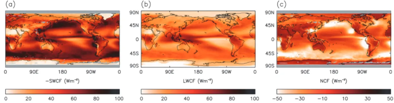
Both longwave and shortwave radiation play an important role in the development of atmospheric processes. They basically determine the temperature distribution in the atmosphere, and thus impact the processes from cloud and precipitation formation on microphysical scale to air mass motion on continental scale. Therefore, many studies have focused on the understanding of radiation budget of the Earth, including, e.g., spatial distribution of cloud- radiation interactions. Large number of these studies have used satellite measurements since the mid-eighties (Ramanathan et al., 1989). They concluded that the global average of shortwave (SW) radiation reaching the surface is reduced by 44.5 W/m2 due to the presence of clouds; and about 31.3 W/m2 is absorbed by the clouds in the longwave (LW) region. Thus, the presence of clouds results in a net decrease of 13.2 W/m2 of total longwave flux.
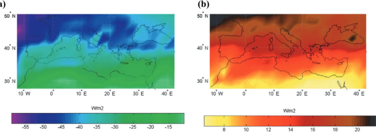
This estimation has been confirmed by contemporary results of the Clouds and the Earth’s Radiant Energy System (CERES) sensors onboard the polar orbiting Terra and Aqua satellites (Allan, 2011). Fig. 1 shows the mean effect of clouds on radiation fluxes in shortwave (a) and longwave (b) range, furthermore, their net impact (c) for a 7 years period. We can observe that the net effect of the clouds varies mainly between −20 W/m2 and 10 W/m2, yielding an average around −10 W/m2 (Fig.1c). Similar results have been provided by numerical simulations. For the Mediterranean Basin, Pyrina et al. (2015) calculated that in the case of outgoing SW radiation, the effect of cloud ranged between −60 and
−10 W/m2 on top of atmosphere; whereas in the case of outgoing LW radiation this effect was between 6 and 22 W/m2 on top of atmosphere (Fig. 2). Their result about the net average of around −21 W/m2, however, overestimates the total net impact of clouds on radiation fluxes observed by CERES. This bias, order of 10 W/m2 between numerical simulations and satellite measurements has been often reported in other publications as well (Fairall et al., 2008).
Fig. 1. CERES satellite data on the effect of clouds on the top of atmosphere (TOA) radiation budget between 2001−2007 in the shortwave (a) and longwave (b) region, and
(a) (b)
Fig. 2. 24-year (1984–2007) model computed cloud radiative effects on the Mediterranian region for shortwave TOA (a) and longwave TOA (b) radiation.
1.1. Longwave radiation and cloud interaction
More precise assessment of the impact of clouds on radiation budget becomes possible by the classification of clouds. It was demonstrated that at the top of the atmosphere, the outgoing longwave radiation is mostly modified by high-level cirrus, nimbostratus, and convective clouds; whereas longwave fluxes at the surface are controlled by low-level altostratus, cumulus, and stratocumulus clouds (McFarlane et al., 2013). Our studies concentrated on stratocumulus clouds as they cover approximately one-fifth of the Earth’s surface as an annual average (Wood, 2012). Moreover, longwave radiation is the main driver to stratocumulus cloud formation and life-cycle; because cooling rates due to large longwave radiation emission at the top of these clouds cause the instability that maintains the convective updraft in stratocumulous clouds. Reduced entrainment because of cooling at cloud top can even result in significant extension of cloud lifetime (Petters et al., 2012). Similarly to stratocumulus clouds, longwave cooling at the top of a fog layer influences significantly the evolution of the fog (Gultepe and Milbrandt, 2007). Also, it is the main factor in mixing with the air above the foggy layer (Mazoyer et al., 2017).
Longwave radiation cooling occurs within a 20−50 m thick layer at the cloud top, and its value varies mainly between −7 K/h and −13 K/h (Austin et
rate of longwave cooling at the top of the cloud and the fog (Wærsted et al., 2017). Therefore, it is important to study the interaction on a microphysical scale containing information of cloud-size distribution. This can only be done by numerical models as radiation measurement campaigns fail to provide sufficient accuracy especially in the case of pyrgeometers (Ackerman et al., 1995).
2. Numerical methods to describe radiation-cloud processes
Numerical weather prediction models apply parameterization tools to simulate physical processes. These parameterizations imply application of simplified mathematical formulas to describe natural phenomena, otherwise it would need large computer capacity and would take very long time to numerically reproduce these processes. In our case, two different parameterizations are considered:
radiation schemes involving calculation of absorption coefficients, and microphysical schemes determining concentration and mixing ratio of water droplets. Thus, enhancement of radiation scheme can be either achieved by enhancement of input parameters from more precise microphysical parameterization (e.g., two-moment or even bin scheme instead of one-moment schemes, Lee and Donner, 2011); or by improvement of radiation absorption parameterization itself. We have developed a method to combine both, that is, we have implemented a method to calculate the absorption coefficients by incorporating the bin microphysical scheme in new equations. This modification is made within the radiative transfer model RRTMG LW (rapid radiative transfer model for the longwave radiation) (Mlawer et al., 1997; Clough et al., 2005), a high accuracy numerical radiation tool implemented in several global numerical weather prediction models like ECMWF (Morcrette et al., 2008) or GFS (Sun et al, 2010), as well as in limited area weather forecasting models like ALADIN (Yessad, 2014) or WRF (Deng et al., 2009). It divides the longwave spectra into 16 bands.
Detailed bin microphysical schemes are characterized by a number of size intervals of the water droplets (in our case, 36), where the concentration and mixing ratio of water droplets are calculated separately; thereofore, arbitrary size distribution of droplets can be converged. Otherwise, in one-moment and two-moment schemes, we need an assumption for the size distribution function, which is normally a gamma-function (Lee and Donner, 2011). These latter approximations are called bulk-schemes.
If size distribution is known, volume absorption coefficients can be calculated by the following formula:
, (1)
βabs ,λ(z ' ')=π
∫
0
∞
n(r , z' ')r2Qabs(λ , r)dr
where n(r,z’’) is the size distribution at location z’’, r is the radius of the droplet, λ is the wavelength, and Qabs is the absorption efficiency (Petty, 2006).
Longwave radiation interaction with clouds includes both absorption and scattering (which together produce longwave extinction). However, the whole process is dominated by the absorption (Delamere et al., 2000) for water droplets; scattering is non-negligible in case of high cirrus clouds (Fu et al., 1997). Since in the RRTMG LW model only absorption coefficients are used for the bulk scheme, in the present publication we have used the bin absorption coefficient to study effects of this new bin radiation scheme for water clouds.
Studies applying the bin extinction coefficient (βext) as approximation for longwave interactions were published in Lábó and Geresdi (2016).
2.1. Bin method to calculate the radiation coefficients
If we use a bin scheme, we have Nbins=36 bins in which different size distributions are labeled as nk(M), and so the volume coefficients can be calculated for a wavelengh interval Δλ as a weighted average according to the Eλ
Planck-function:
, (2) where Mk-1 and Mk are the mass of droplets at the edges of the kth bin, A(D) is the cross section (A(D) = π r2), D is the diameter of droplet, and m is the refraction index.
In bulk numerical models, the absorption coefficients are given by an empirical formula, such as:
= ∙ + , (3)
where a, b, and c coefficients are fixed according to empirical data; and can be evaluated for different size-intervals of water drops (Hu and Stamnes, 1993).
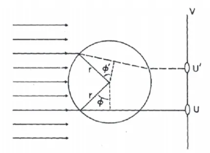
Nevertheless, it is possible to solve Eq.(2) if Qabs is given by analytical formula. For this, we have used the Modified Anomalous Diffraction Theory (MADT, Mitchell, 2000). The MADT approximation is based on the propagation of electromagnetic waves as it is plotted in Fig. 3.
βabs=
∑
k=2 Nbins
[
∫
∆λ
Eλ
∫
Mk−1
Mk
A(D)Qabs(D , m ,λ )nk (M)dMdλ/
∫
∆λ
Eλdλ]
Fig. 3. Trajectories of incoming electromagnetic wave on a water droplet symbolized by the circle (Ackerman and Stephens, 1987).
In addition to absorption coefficients calculated by the Anomalous Diffraction Theory method (Qext,ADT), the MADT method also takes into account reflection and refraction (Cres) of the electromagnetic waves, and the correction for internal reflection and refraction (Cir):
. (4) The MADT method provides analytical formulas for Qabs as a function of D, λ, and m (Harrington and Olson, 2001). If we put these equations into Eq.(2), along with the linear formula for the size distribution of the number concentration in the kth bin ( ) = + ∙ , we have the following expression for βabs:
= ∑ ∙ ∑ ( , , ∆ ) + ∑ ∙ ∑ ( , , ∆ ).(5)
In Eq.(5), j denotes the band (and Δλj is the bandwidth) used in the RRTMG LW model.
Because the elements of KAkj(Mk-1,Mk,Δλj) and KBkj(Mk-1,Mk,Δλj) matrixes can be pre-calculated (without knowing the actual nk(M) distribution itself) and the Ak and Bk coefficients are evaluated by the microphysics scheme, the βabs can be calculated very efficiently (Lábó, 2017).
Qabs(D ,λ , m)= (1+Cir(D ,λ , m)+Cres(D ,λ , m))Qabs , ADT(D ,λ , m)
3. Comparison of results for the two schemes
Before application of the new scheme with the RRTMG LW radiation transfer model for a stratocumulus cloud, we have compared solely the bulk and bin absorption coefficients that will be used in the RRTMG model.
3.1. Comparison of longwave absorption coefficients evaluated by bulk and bin schemes
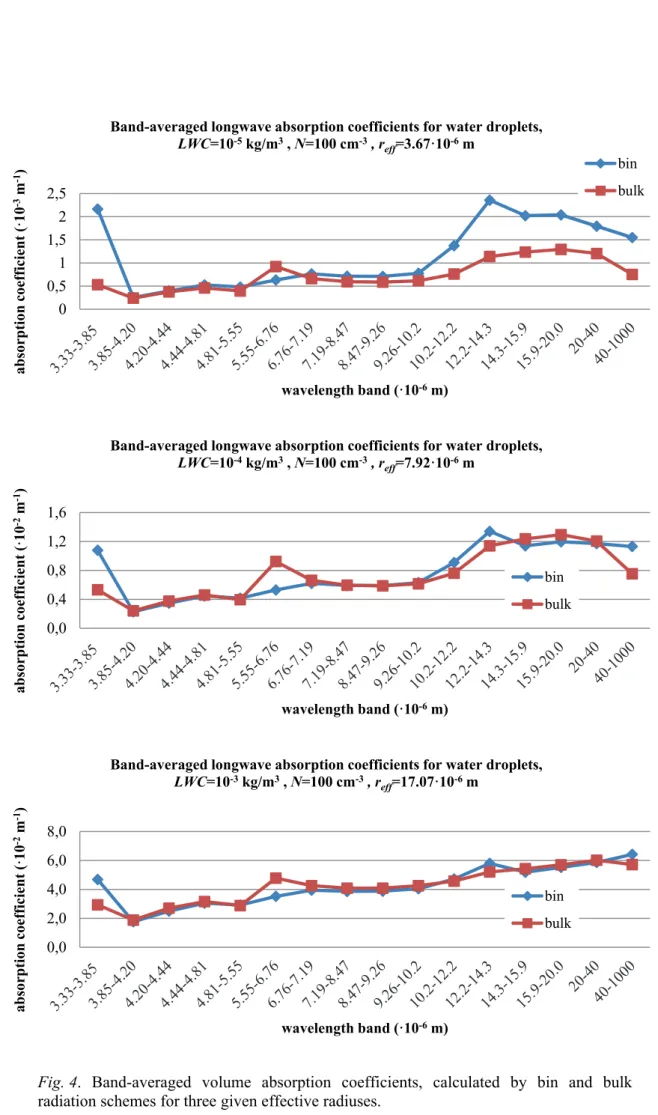
The absorption coefficients caculated by current bin scheme (using Eq.(5)) are compared to that of calculated by bulk scheme using Eq.(3) (Hu and Stamnes, 1993). The absorption coefficients averaged over the wavelenght-bands defined in RRTMG LW model were compared (Fig. 4). The bulk data can be found in the lookup table of RRTMG LW model, bin data were calculated by using Eq.(5). The comparison of the plots shows that variations between these absorption coefficients are higher mainly in case of smaller effective radius (reff < 5 µm) and at larger wavelenghts (> 10 μm). The difference reaches a factor of 2 around 10 μm (close to the peak of the Planck-function), out of this interval the divergence decreases rapidly. For larger effective radius (reff ~ 8 µm) the differences are significantly smaller (maximum 20%). Large deviation occurs only in the band of 5.55–6.76 µm, however, at these wavelenghts the value of Planck function is low.
Besides the absorption coefficients, we have compared the extinction coefficients for individual wavelengths in our previous study, published in Lábó and Geresdi (2013). In that study, similar results were found: the difference between the extinction coefficients based on the bulk and bin schemes was relatively small, about 10–20% if reff < 12 µm, and even smaller (< 10%) for the larger effective radius.
Fig. 4. Band-averaged volume absorption coefficients, calculated by bin and bulk radiation schemes for three given effective radiuses.
0 0,5 1 1,5 2 2,5
absorption coefficient (·10-3m-1)
wavelength band (·10-6m)
Band-averaged longwave absorption coefficients for water droplets, LWC=10-5kg/m3, N=100 cm-3, reff=3.67·10-6m
bin bulk
0,0 0,4 0,8 1,2 1,6
absorption coefficient (·10-2m-1)
wavelength band (·10-6m)
Band-averaged longwave absorption coefficients for water droplets, LWC=10-4kg/m3, N=100 cm-3, reff=7.92·10-6m
bin bulk
0,0 2,0 4,0 6,0 8,0
absorption coefficient (·10-2m-1)
wavelength band (·10-6m)
Band-averaged longwave absorption coefficients for water droplets, LWC=10-3kg/m3, N=100 cm-3, reff=17.07·10-6m
bin bulk
3.2. New results for longwave heating rates
The band-averaged bin absorption coefficients were implemented in the RRTMG LW radiative transfer model (named bin radiation scheme in the present publication). The results of this bin radiation scheme were compared to the results of initial RRTMG LW bulk scheme. The original version of RRTMG LW (called bulk radiation scheme in the present publication) uses Eq.(3) in computing the absorption coefficient.
A two-dimensional kinematic model was used to simulate the formation of shallow stratocumulus clouds. In this model, a detailed bin microphysical scheme was applied (Lábó and Geresdi, 2016) to prepare the vertical profile of the liquid drops for application in the bin radiation scheme. Vertical transfer of longwave radiation was calculated in each vertical column throughout a domain which included the cloud. The domain had an extent of 2 km horizontally and 1 km vertically, and a grid resolution of 20 m in both directions.
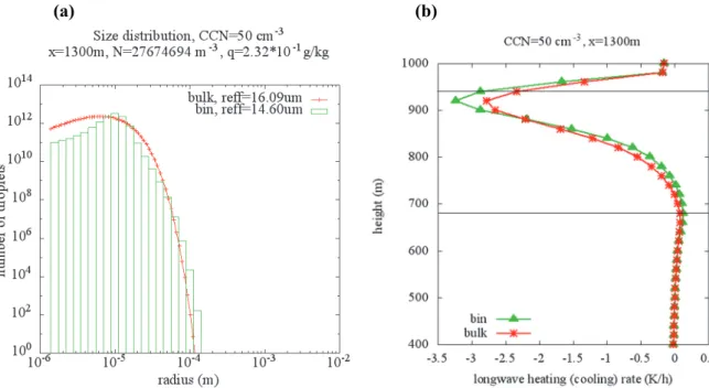
Fig. 5a shows the size distributions related to the bin and bulk microphysical schemes in one of the grid points in the downdraft region of the cloud; furthermore, Fig.5b shows the calculated longwave heating rates in the column containing this grid point. It can be observed that the bin cooling rate is higher at the cloud top, as well as the bin heating rate is higher at the cloud base than the bulk rates. The differences are about 20% at both for cloud top and base. Note that cooling occurs in a narrower layer in the case of the bin scheme.
Similar results for the bin radiation scheme compared to the bulk scheme were found for higher CCN concentrations (Lábó and Geresdi, 2016). Contrary to the comparison of the absorption coefficients (Fig. 4), for which we have assumed that the size-distributions of water droplets are the same for both bulk and bin schemes, the two microphysical schemes applying different description of the microphysical processes resulted in distinct size distributions (see Fig. 5a). This difference must have contributed to the divergence between the heating/cooling rates calculated by the two schemes.
(a) (b)
Fig. 5. Size distribution and effective radius in a given grid point of the stratocumulus cloud (a); and vertical longwave flux profiles in the same column(x=1300 m) (b); for the bin and bulk radiation schemes. The horizontal lines show the cloud top and base.
Fig. 6 shows the 2D cross section of the evaluated cooling rates in case of a maritime stratocumulus cloud if cloud condensation nuclei conentration was equal to 100 cm-3 (CCN=100 cm-3).
Comparison of Fig. 6a and Fig. 6b shows that the bin longwave cooling rates at cloud top always exceed the rates calculated by the bulk scheme (Fig. 6c). This cooling occurs in a thinner layer in the case of bin scheme (about 80 m) than in the case of bulk scheme (about 100 m). The heating rate at cloud base is also slightly larger in the case of bulk scheme. The difference between the highest cooling rates remains around 20%.
(a)
(b)
(c)
3.3. Comparison with longwave cooling rates in other studies
Measurement of longwave cooling rates in stratocumulus clouds has always been a challenging task, which demonstrated large uncertainties of the measurements of radiation fluxes by Eppley pyrgeometers (±10 W/m2) (Duda et al., 1991). Therefore, from the nineties, cooling rates were derived mostly by numerical modeling simulations. These studies dealt with clouds formed over maritime areas (as 80% of stratocumulus clouds occur in these regions), so we have used the results of numerical simulations of condensation nuclei concentration of CCN=100 cm-3 for comparison.
Because longwave cooling rates strongly depend on the liqiud water concentration (LWC) profiles (Lábó and Geresdi, 2016), the maximum liquid water contents are also summarized in Table 1.
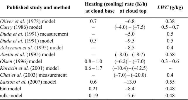
Table 1. Comparison of values of longwave cooling rates at cloud base and cloud top of maritime stratocumulus (CCN~100 cm3)in different publications, and results for the CCN100 cloud in our studies (bin and bulk shemes)
Published study and method Heating (cooling) rate (K/h)
at cloud base at cloud top LWC (g/kg)
Oliver et al. (1978) model 0.7 –6.8 0.38
Curry (1986) model – (–4.0) – (–7.5) 0.5–0.7
Duda et al. (1991) measurement – –5.0 0.5
Duda et al. (1991) model 0.5 –9.5 0.5
Ackerman et al. (1995) model – –8.5 0.4
Austin et al. (1995) model – (–8.0)–(–8.7) 0.58 Olsen (1996) model 0.8–1.0 (–6.2) – (–7.0) 0.3–0.6 Koracin et al. (2001) model 0.6–1.7 (–10.4)–(–12.5) – Chai et al. (2003) measurement – (–7.0)–(–20.0) 0.4
Larson et al. (2007) model 0.6 –13.0 0.55
bin model 0.21 –8.4 0.48
bulk model 0.19 –7.6 0.48
It can be seen from Table 1, that the simulated heating rates at cloud base for both of our bin and bulk simulations are lower than that of the published values. However, the bin values are a bit (+10%) closer to these results. For the cloud top cooling rates, we can see that the bulk result (−7.6 K/h) is in better agreement with the values published before the 90s, as they are as well below
−8 K/h. Contrary, the bin result (−8.4 K/h) is more in line with recently reported values, as these values mostly exceed 8 K/h in terms of absolute rate.
It has to be noted as well, that there is a large variance in the values of cooling rates published in Table 1., which is much higher that the difference observed between the bin and bulk shemes (~10%). Nevertheless, it can be stated that there is a persistent underestimation of the published rates by the bulk scheme; whereas the bin scheme gives a rate well within the range of dispersion of the reported values. The extremes of the cooling rates at cloud top are recorded by those studies based on measurements: Duda et al. (1991) gives the lowest, and Chai et al. (2003) gives the highest number in absolute terms. This can be explained by the large errors due to observation equipment (pyrometers, Stevens et al., 2003). In addition, the reason for this deviance might be in Duda et al. (1991) that they supposed that the shapes of net flux profiles in the clouds are similar even if liquid water contents are different, which is not correct (Lábó and Geresdi, 2016).
We also have to emphasize that the depth of the cooling layer at cloud tops is widely accepted to be between 20–50 m (Ackerman et al. 1995; Bergot et al., 2007). In Figs. 6a and b, it is illustrated that the bin and bulk schemes both overestimate this range; nonetheless, the bin value is slightly closer (~80 m).
4. Application of the bin radiation scheme for fog
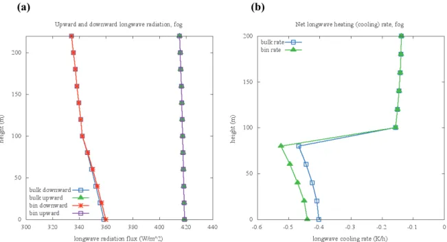
Whereas the liquid water content is around 0.5 g/kg in stratocumulus clouds, fogs contain less water, typically between 0.01 and 0.4 g/kg, with effective radius varying from 4 to 10 µm (Chai et al., 2003; Gultepe and Milbrandt, 2007). As a result of lower LWC, longwave radiation profiles show a different profile inside the fog layer. We have examined this by assuming idealized gamma-profiles for both the bin and bulk schemes within a 1D fog layer, where the liquid water content was constant (0.1 g/kg), and the thickness of the layer was 100 m. The results of the simulations accomplished by the RRTMG LW model can be seen in Fig. 7.
(a) (b)
Fig. 7. Upward, downward (a) longwave radiation profiles and the cooling rates (b) in a fog layer for the bin and bulk radiation schemes.
We can see in Fig. 7a. that the difference of the net flux between the bin and bulk schemes at the surface is around ~1.5 W/m2, which is the consequence of larger absorbence by the bin method in the downward direction. The resulting maximum cooling rate within the cloud is −0.53 K/h for the bin scheme, and
−0.47 K/h for the bulk scheme; which gives a total of 12% difference in the cooling rate. These rates are lower than published in Koracin et al. (2001) or Wærsted et al. (2017), as they both studied fogs with much higher (0.3–0.4 g/kg) liquid water content.
Because of the difference in bin and bulk rates, the absorption changes stronger with the altitude in case of the bin method, thus a more pronounced temperature inversion will form when using the bin model in a dynamical setting (Gultepe et al., 2007), which helps the fog to persist. Thus, longer lifetime of the fog can be predicted by the bin scheme in cold pool situations. Moreover, if the fog prevails, the energy balance at the surface is lower, as every minute
~90 W/m2 less energy reaches the ground in case of the bin scheme; which will considerably impact the soil-atmosphere interaction processes.
5. Conclusions
A new bin radiation scheme related to a bin microphysical scheme has been developed, and results about its application by using the RRTMG LW longwave radiation-transfer model are presented. The MADT approximation was used for calculation of radiation-water drop interaction in the new scheme to produce the bin longwave absorption coefficients for water clouds. The dependence of the coefficients on the wavelength confirmed that coefficients related to the bin scheme are in tune with the results of a so-called bulk radiation scheme currently used in operational numerical weather prediction models.
However, bin radiation scheme gave stronger radiation cooling rate than the bulk scheme at the top of the stratocumulus cloud. This distinction between the two schemes can be explained, partly, by the different approximation techniques used for calculation of absorption coefficients and mainly due to the different size distributions used in the two schemes. Even if same size distribution of water droplets was used in case of a fog layer, the cooling rates showed a divergence of 12%. We have also concluded that results of the new bin radiation scheme for marine stratocumulus clouds are improved compared to the bulk outcomes, as they are both closer to other published values of cooling/heating rates and those of depth of cooling region at cloud top.
The new method can currently be applied in simulations of fog occurrence and prediction of the lifetime of fog and water clouds. All numerical weather prediction models and their research versions which incorporate the RRTM LW radiation model are capable to use this new bin longwave radiation scheme, if number concentrations of water droplets in bin intervals are available as prognostic variable in the model. In such a case, the new radiation scheme does not require further computing resources. The new method can also be extended to other radiative transfer models, by calculation of relevant coefficients for the wavelength bands of the given radiative model.
Acknowledgements: The present study was supported by the Economic development and innovation operational program (project number: GINOP 2.3.2-15-2016-00055).
References
Ackerman, A.S., Toon, O.B., and Hobbs, P.V., 1995: A Model for Particle Microphysics, Turbulent Mixing, and Radiative Transfer in the Stratocumulus-Topped Marine Boundary Layer and
Bergot, T., Terradellas, E., Cuxart, J., Mira, A., Liechti, O., Mueller, M., and Woetmann, N., 2007:
Intercomparison of Single-Column Numerical Models for the Prediction of Radiation Fog. J.
Appl. Meteorol. Climatol., 46, 504–521. https://doi.org/10.1175/JAM2475.1
Chai, S. K., Wetzel, M. A., and Koracin, D., 2003: Observed Radiative Cooling in Nocturnal Marine Stratocumulus. Fifth Conf. Coast. Atmos. Ocean. Predict. Process.
Clough, S.A., Shephard, M.W., Mlawer, E.J., Delamere, J.S., Iacono, M.J., Cady-Pereira, K., Boukabara, S., and Brown, P. D., 2005: Atmospheric Radiative Transfer Modeling: A Summary of the AER codes, Short Communication. J. Quant. Spectrosc. Radiat. Transf., 91, 233–244.
https://doi.org/10.1016/j.jqsrt.2004.05.058
Curry, J.A., 1986: Interactions among Turbulence, Radiation and Microphysics in Arctic Stratus Clouds. J. Atmos. Sci., 43, 90–106.
https://doi.org/10.1175/1520-0469(1986)043<0090:IATRAM>2.0.CO;2
Delamere, J.S., Mlawer, E.J., Clough, S.A., and Stamnes, K.H., 2000: The impact of cloud optical properties on longwave radiation in the Arctic. In Tenth ARM Sci. Team Meet. Proc., San Antonio, Texas.
Deng, A., Stauffer, D., Gaudet, B., Dudhia, J., Hacker, J., Bruyere, C., Wu, W., Vandenberghe, F., Liu Y., and Bourgeois, A., 2009: Update on WRF-ARW end-to-end multi-scale FDDA system. 10th Annu. WRF users’ workshop.
http://www2.mmm.ucar.edu/wrf/users/workshops/WS2009/presentations/1-09.pdf
Duda, D.P., Stephens, G.L., and Cox, S.K., 1991: Microphysical and Radiative Properties of Marine Stratocumulus from Tethered Balloon Measurements. J. Appl. Meteorol., 30, 170–186.
https://doi.org/10.1175/1520-0450(1991)030<0170:MARPOM>2.0.CO;2
Fairall, C.W., Uttal, T., Hazen, D., Hare, J., Cronin, M.F., Bond, N., and Veron, D.E., 2008:
Observations of Cloud, Radiation, and Surface Forcing in the Equatorial Eastern Pacific. J.
Clim., 21, 655–673. https://doi.org/10.1175/2007JCLI1757.1
Fu, Q., Liou, K.N., Cribb, M.C., Charlock, T.P., and Grossman, A., 1997: Multiple scattering parameterization in thermal infrared radiative transfer. J. Atmos. Sci. 54, 2799–2812.
https://doi.org/10.1175/1520-0469(1997)054<2799:MSPITI>2.0.CO;2
Gultepe, I. and Milbrandt, J.A., 2007: Microphysical Observations and Mesoscale Model Simulation of a Warm Fog Case During FRAM Project. Pure Appl. Geophys. 164, 1161–1178.
https://doi.org/10.1007/s00024-007-0212-9
Harrington, J. and Olsson, P.Q., 2001: A Method for the Parameterization of Cloud Optical Properties in Bulk and Bin Microphysical Models. Implications for Arctic Cloudy Boundary Layers.
Atmos. Res., 57, 51–80. https://doi.org/10.1016/S0169-8095(00)00068-5
Hu, Y.X. and, Stamnes, K., 1993: An Accurate Parameterization of the Radiative Properties of Water Clouds Suitable for Use in Climate Models. J. Clim., 6, 728–742.
https://doi.org/10.1175/1520-0442(1993)006<0728:AAPOTR>2.0.CO;2
Koracin, D., Lewis, J., Thompson, W.T., Dorman, C.E., and Businger, J.A., 2001: Transition of Stratus into Fog along the California Coast: Observations and Modeling. J. Atmos. Sci. 58, 1714–1731.
https://doi.org/10.1175/1520-0469(2001)058<1714:TOSIFA>2.0.CO;2
Lábó E. and Geresdi I., 2013: Application of a Detailed Bin Scheme in Longwave Radiation Transfer Modeling. Időjárás 117, 377–402.
Lábó E. and Geresdi I., 2016: Study of Longwave Radiative Transfer in Stratocumulus Clouds by Using Bin Optical Properties and Bin Microphysics Scheme. Atmos. Res. 167, 61–76.
https://doi.org/10.1016/j.atmosres.2015.07.016
Lábó E., 2017: A hosszúhullámú sugárzás stratocumulus felhőben történő terjedésének numerikus modellezése, PhD dissertation, ELTE University, https://edit.elte.hu/xmlui/handle/10831/35125.
(In Hungarian)
Larson, V.E., Kotenberg, K.E., and Wood, N.B., 2007: An Analytic Longwave Radiation Formula for Liquid Layer Clouds. Mon. Weather Rev. 135, 689–699. https://doi.org/10.1175/MWR3315.1 Lee, S.S. and Donner, L.J., 2011: Effects of Cloud Parameterization on Radiation and Precipitation: A
Comparison between Single-Moment Microphysics and Double-Moment Microphysics. Terr.
Atmos. Ocean. Sci. 22, 403–420. https://doi.org/10.3319/TAO.2011.03.03.01(A)
Mazoyer, M., Lac, C., Thouron, O., Bergot, T., Massonv, V., and Musson-Genon, L., 2017: Large eddy simulation of radiation fog: impact of dynamics on the fog life cycle. Atmos. Chem. Phys 17 , 13037-13035. https://doi.org/10.5194/acp-17-13017-2017
McFarlane, S.A., Long, C.N., and Flaherty, J., 2013: A Climatology of Surface Cloud Radiative Effects at the ARM Tropical Western Pacific Sites. J. Appl. Meteorol. Climatol. 52, 996–1013.
https://doi.org/10.1175/JAMC-D-12-0189.1
Mitchell, D.L., 2000: Parameterization of the Mie Extinction and Absorption Coefficients for Water Clouds. J. Atmos. Sci. 57, 1311–1326.
https://doi.org/10.1175/1520-0469(2000)057<1311:POTMEA>2.0.CO;2
Mlawer, E.J., Taubman, S.J., Brown, P.D., Iacono, M.J., and Clough, S.A., 1997: Radiative Transfer for Inhomogeneous Atmospheres: RRTM, A Validated Correlated-k Model for the Longwave.
J. Geophys. Res., 102(D14), 16,663–16,682. https://doi.org/10.1029/97JD00237
Morcrette, J.-J., Barker, H., Cole, J., Iacono, M., and Pincus, R., 2008: Impact of a new radiation package, McRad, in the ECMWF Integrated Forecasting System. Mon. Weather Rev. 136, 4773–4798. https://doi.org/10.1175/2008MWR2363.1
Oliver, D.A., Lewellen, W.S., and Williamson, G.G., 1978: The Interaction between Turbulent and Radiative Transport in the Development of Fog and Low-Level Stratus. J. Atmos. Sci., 35, 301–316.
https://doi.org/10.1175/1520-0469(1978)035<0301:TIBTAR>2.0.CO;2
Olsen, L.D., 1996: Analysis of Infrared Heating Rates in Observed Cloud Layers. M. S. Thes., Colo.
State Univ., Dept. of Atmos. Sci., Fort Collins. 620.
Petters, J.L., Harrington, J.Y., and Clothiaux, E.E., 2012: Radiative–Dynamical Feedbacks in Low Liquid Water Path Stratiform Clouds. J. Atmos. Sci., 69, 1498–1512.
https://doi.org/10.1175/JAS-D-11-0169.1
Petty, G.W., 2006: A First Course in Atmospheric Radiation. Madison, Wis., Sundog Pub.
Pyrina, M., Hatzianastassiou, N., Matsoukas, C., Fotiadi, A., Papadimas, C.D., Pavlakis, K.G., and Vardavas, I., 2015: Cloud Effects on the Solar and Thermal Radiation Budgets of the Mediterranean Basin. Atmos. Res., 152, 14–28. https://doi.org/10.1016/j.atmosres.2013.11.009 Ramanathan, V., Cess, R.D., Harrison, E.F., Minnis, P., Barkstrom, B.R., Ahmad, E., and Hartmann, D.,
1989: Cloud-Radiative Forcing and Climate: Results from the Earth Radiation Budget Experiment.
Science, New Series., 243, 4887, 57–63. https://doi.org/10.1126/science.243.4887.57
Stevens, B., Lenschow, D.H., Vali, G., Gerber, H., Bandy, A., Blomquist, B., Brenguier, J.-L., Bretherton, C.S., Burnet, F., Campos, T., Chai, S., Faloona, L., Friesen, D., Haimov, S., Laursen, K., Lilly, D.K., Loehrer, S.M., Malinowski, S.P., Morley, B., Petters, M.D., Rogers, D.
C. Russell, L., Savic-Jovcic, V., Snider, J.R., Straub, D., Szumowski, M.J., Takagi, H., Thornton, D.C., Tschudi, M., Twohy, C., Wetzel, M., and van Zanten, M.C. , 2003: Dynamics and chemistryof marine stratocumulus—DYCOMS-II. Bull. Amer. Meteor. Soc., 84, 579–593.
https://doi.org/10.1175/BAMS-84-5-Stevens
Sun, R., Moorthi, S., Xiao, H., and Mechoso, C.R., 2010: Simulation of low clouds in the Southeast Pacific by the NCEP GFS: sensitivity to vertical mixing. Atmos. Chem. Phys. 10, 12261–12272.
https://doi.org/10.5194/acp-10-12261-2010
Wærsted, E.G., Haeffelin, M., Dupont, J.-C., Delanoë, J., and Dubuisson, P.: Radiation in fog:
quantification of the impact on fog liquid water based on ground-based remote sensing. Atmos.
Chem. Phys. 17, 10811–10835. https://doi.org/10.5194/acp-17-10811-2017 Wood, R., 2012: Stratocumulus Clouds. Mon. Weather Rev., 140(8), 2373-2423.
https://doi.org/10.1175/MWR-D-11-00121.1
Yessad, K., 2014: Basics about ARPEGE/IFS, ALADIN and AROME in the cycle 41 of ARPEGE/IFS. http://www.cnrm.meteo.fr/gmapdoc/IMG/pdf/ykarpbasics41.pdf, 2014