IDŐJÁRÁS Quarterly Journal of the Hungarian Meteorological Service

DOI:10.28974/idojaras.2018.1.4

IDŐJÁRÁS

Quarterly Journal of the Hungarian Meteorological Service Vol. 122, No. 1, January – March, 2018, pp. 41–58

Estimation of natural water body’s evaporation based on Class A pan measurements in comparison to reference

evapotranspiration

Angéla Anda*, Brigitta Simon, Gábor Soós, and Tamás Kucserka

Department of Meteorology and Water Management, Georgikon Faculty, University of Pannonia, Festetics Str. 7. Keszthely, H-8360, Hungary

*Corresponding author E-mail:anda-a@georgikon.hu (Manuscript received in final form March 21, 2017)

Abstract⎯ A Class A pan (C) evaporation (Ep) study was conducted at the Agrometeorological Research Station of Keszthely, in the growing season of 2016. Some of the evaporation pans were implemented with freshwater aquatic macrophytes (Myriophyllum sp., Potamogeton sp., and Najas sp.) (Ps) and sediment covered bottom (S).

The applied macrophytes were the predominant species of Keszthely Bay (Balaton Lake).

Reference (Eo) after Shuttleworth and reference evapotranspiration (ETo) after Penman- Monteith (FAO-56 formula) were also included for the E study. Of pre-selected four investigated variables, air temperature and air humidity impacted Ep of treated Class A pans the most. Cumulative Ep values for 2016 were 363.1, 427.7, and 461.5 mm in C, S, and Ps, respectively. There was no difference in measured cumulative Ep of Ps (461.5 mm) and computed ETo (472.1 mm) during the studied season.

On the basis of a simplified water budget, E rate of Keszthely Bay increased with 16.9%, when macrophytes and sediment cover were accounted. It is equivalent to 264,000,000 m³ water in Keszthely Bay’s E estimation. Simple E approach - when lake’s components, such as submerged macrophytes and sediment cover were also accounted - could extend the accuracy of natural lake’s E estimation in a broader circle than earlier.

Key-words: Class A pan evaporation, aquatic macrophytes, Keszthely Bay (Balaton Lake)

1. Introduction

Evaporation (E) is the process of conversion of liquid water to water vapor, widely measured by standard dish filled with water. Evaporation pans provide a measurement of the integrated influence of temperature, humidity, wind speed, and solar radiation on E (Majidi et al., 2015; Kim et al., 2013). In the last century, due to its cost-effectiveness and easy-applicability, pan evaporation (Ep) measuring network has been established worldwide (Stanhill, 2002). The physical basis of Class A pan’s Ep was investigated among others by Roderick et al. (2007) and Jacobs et al. (1998). Ep has also been applied as an index of lake and reservoir E (Wang et al., 2017; Kim et al., 2015; Allen et al., 1998) beyond traditional Ep

uses in water budget estimation, plant-weather interactions, etc. Spatial and temporal limitations of pan application due to instrumental and practical issues were also integrated (Martí et al., 2015; Shiri et al., 2011). Several empirical methods based on local variables, in many cases various meteorological drivers, have been developed to estimate Ep in different climate conditions. Weaknesses in use of empirical or half-empirical equations may be the limited data availability and completeness (Majidi et al., 2015). The other option in E estimation is the modeling approach, the Penman-Monteith reference evapotranspiration (ETo) model (Allen et al. 1998, 2005; FAO-56 equation) is probably the most widely employed method among E approximations.

Linacre (1994) issued that Ep does not correspond well to open-water E due to modified intercepted radiation and enhanced heat exchange of the pan wall. To manage issues of A pan’s heat transfer modifications, a pan coefficient (below unity) is in use to get near-natural E values (Allen et al. 1998; Linacre, 1994). In addition to radiation and heat transfer variations, Rotstayn et al. (2006) identified aerodynamic deviations in pan’s physical behavior. Recognizing fragility of our knowledge in physical properties of pans, Yang and Yang (2012) found that E pans are not desirable in open-water E estimations. Lim et al. (2012) collected the most frequent sources of errors when Class A pan is used: the upper thin layer’s surface temperature declines due to evaporation, unknown water mixing inside the dish, experimental shortcomings of some researchers, etc. (Anda et al., 2016).

The term macrophyte comprises plants which are at least with their roots under water (Barrat-Segretain, 1996). One of the three sub-groups of macrophytes (emergent, floating leaved, and submerged) is the submerged one, which keep their leaves permanently under water. Brothers et al. (2013) found that submerged macrophytes are the key factors in aquatic ecosystems as they strongly impact lake productivity. Another important role of submerged macrophytes is their contribution to clear-water conditions of shallow lakes and rivers (Hilt et al., 2011).Three predominant submerged macrophyte species are present at Keszthely Bay (Balaton Lake): Myriophyllum sp., Potamogeton sp., and Najas sp. (Vári, 2012).

There are not any studies in the literature that account impact of sediments and submerged macrophytes in estimating lake’s E. Information deficit related to living water E approach, when class A pan is in use, might impede for the present measurement of a more accurate E estimation.

2. Materials and methods

2.1. Study site and pan treatments with E estimations

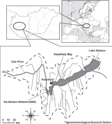
Class A pan’s Ep observations were carried out at the Keszthely Agrometeorological Research Station (latitude: 46° 44ʹ N, longitude: 17° 14ʹ E, elevation: 124 m above sea level) in the growing season of 2016 (Fig. 1). Three different pan treatments were set in the study:

− Class A pan as control pan (C),

− Class A pan implemented with submerged macrophytes (Ps),

− Class A pan with sediment covered bottom (S).

Fig. 1. Watershed of the Balaton Lake with the site of the observation. Meteorological observations with pan evaporation measurements were done at the Agrometeorological Research Station.

Operation of Class A pan, placed on a 0.15 m high wooden platform, was performed following a standard procedure given by the Hungarian Meteorological Service. After daily water height observations carried out at 7.00 am, water replenishing was executed with tap water. Water temperature, Tw at a depth of 0.02 m was measured with thermocouples at 10 min intervals. Ep observations were only carried out during the growing season.

Predominant submerged freshwater macrophytes (Myriophyllum sp., Potamogeton sp., Najas sp.) were implemented into the Class A pan on June 6, 2016, at the same time when the species emerged in the Balaton Lake (Keszthely Bay). The amount and species distribution of plant samples were consistent with plant density of the Keszthely Bay. Fresh weight of samples was determined at the pan’s seeding time (spring) and in the end of E measurements, on September 30, 2016. Thickness of sediment on the bottom of Class A pan was 0.02 m.

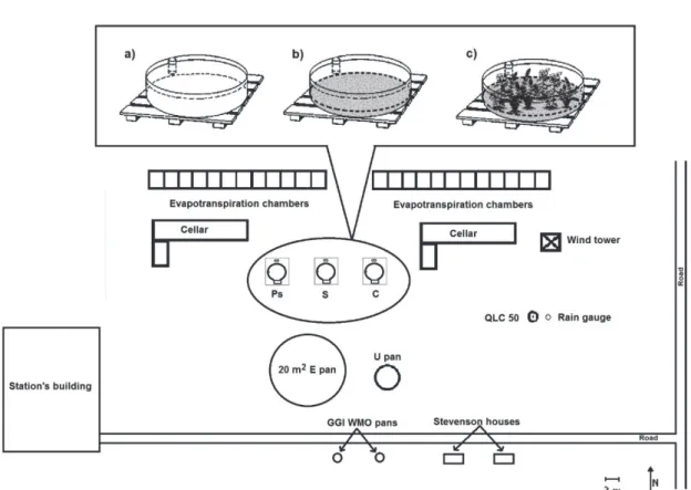
Sediment was obtained from the Balaton Lake. The layout of the pan treatments and instruments of the meteorological station included in the study are presented in Fig. 2.

Fig. 2. Layout of the evaporation pans with the sketch of instrumentation of the Agrometeorological Research Station at Keszthely.

Daily Eo rate [mm day^–1] of water bodies was computed by the Shuttleworth formula (Shuttleworth, 1993), which was adapted from the original Penman equation (Penman, 1948):

= ^{∗ . ( . ∗ )}

( ) , (1)

where Rn is net radiation [MJ m^–2 day^–1], m is the slope of the saturation vapor pressure curve [kPa K^–1], u2 is wind speed [m s^–1] at 2 m height, δe is the vapor pressure deficit [kPa], λv is the latent heat of vaporization [MJ kg^–1], and γ is a psychrometric constant [kPa °C^–1].

Daily plant ETo rate [mm day^–1] was computed by the widely spread FAO- 56 Penman-Monteith equation (Monteith, 1965; Penman, 1948):

= ^{. ( ) ( )}

( . ) , (2)

where G is the soil heat flux density [MJ m^–2 day^–1], Ta is the mean daily air temperature at 2 m height [°C], es is the saturation vapor pressure [kPa], ea is the actual vapor pressure [kPa], Δ is the slope of the vapor pressure curve [kPa °C^–1] and 0.408 is the a conversion factor from MJ m^–2 day^–1 to equivalent evaporation in mm day^–1. Rn was the estimated using the sediment covered bottom treatment (S), from daily mean Ta, mean daily ea, the site latitude and elevation after Allen et al.

(2005). A fixed value of 0.23 was applied for albedo. Rn was also computed after Allen et al. (2005). Detailed description of the way of Rn computation can be read in Soos and Anda (2014) as follows:

Rn is the difference between the incoming net shortwave (Rns) and the outgoing net longwave radiation (Rnl):

Rn = Rns – Rnl . (3)

The net solar or shortwave radiation, Rns [MJ m^–2 day^–1] is given by:

Rns = (1–α)Rs , (4)

where α is the albedo for the reference crop. The incoming solar radiation, Rs [MJ m^–2 day^–1] was measured locally by a CM-3 pyranometer.

Net longwave (outgoing) radiation, Rnl [MJ m^–2 day^–1] was calculated as follows:

[

]

=

SO S a

K mean

nl R

e R T

R σ , (5)

where σ is the Stefan-Boltzmann constant [ 4.903 10^–9 MJ K^–4 m^–2 day^–1], Tmean,K

is the mean temperature during the 24-hour period [K], Rs/Rso is the relative shortwave radiation (limited to ≤ 1.0), Rs is the measured solar radiation [MJ m^–2 day^–1], Rso is the calculated clear-sky radiation [MJ m^–2 day^–1].

To get clear-sky solar radiation Rso [MJ m^–2 day^–1], the station elevation is required:

= (0.75 + 2 ∗ 10 ) , (6)

where Ra is the extraterrestrial radiation [MJ m^–2 day^–1].

Ra, [MJ m^–2 day^–1] is calculated by:

= ^{( )} sin( ) sin( ) + cos( ) cos( ) sin( ) , (7) where Gsc is the solar constant = 0.0820 MJ m^–2 min^–1, dr is the inverse relative distance between the Earth and Sun, δ is the solar declination [rad], ωs is the sunset hour angle [rad], φ is the latitude [rad] at Keszthely.

The lacking parametrs are calculated as follows:

= 1 + 0.033 cos . (8)

= 0.409 sin − 1.39 , (9)

where J is the number of the day in the year between 1 (January 1) and 365 or 366 (December 31).

The sunset hour angle, ωs, is given by:

= − tan( ) tan( ) . (10)

As the magnitude of the day or ten-day soil heat flux beneath the grass reference surface is relatively small, it may be ignored, and thus (Allen et al., 2005):

Gday ≈0 . (11)

Class A pan’s coefficients (K) were derived from the measured Ep of S (Ks) and Ps (Kp), and the control Class A pan Ep:

= , (12)

= . (13)

Weather conditions

Weather variables were recorded by a QLC-50 climate station (Vaisala, Helsinki, Finland) equipped with a CM-3 pyranometer (Kipp & Zonen Corp., Delft, the Netherlands). The combined Ta and humidity sensors were placed at a standard height (2 m above the soil surface). Signals from meteorological elements were collected every 2 second, and 10 minute means were logged by the station. The height of the anemometer was 10.5 m.

The wind speed was adjusted to standard height, u2, [m s^–1] of 2 m:

= _{( .} ^. _{. )} , (14)

where uz is the measured wind speed at 10.5 m above the ground surface [m s^–1], zm is the height of measurement above the ground surface (10.5 m).

The weather conditions of the studied months were specified by the monthly Thornthwaite index, TI of the World Meteorological Organisation (WMO, 1975):

=1.65(P/Ta+12.2)^10/9 (15)

where P and Ta are the monthly sum of precipitation and the monthly mean air temperature, respectively.

In classifying the weather conditions in each season’s months, a 20%

deviation was assumed from the climate normals (1971–2000), above and below the TInorm for both included meteorological variables (P and Ta), allowing the following weather classes to be distinguished (Anda et al., 2014):

warm-dry month (h): TI month > TI norm × 0.8;

cool-wet month (c): TI month > TI norm × 1.2;

month with normal weather (n): TI norm × 0.8 ≤ TI month ≤ TI norm × 1.2.

By counting the highest number of months within each of these three groups, the season was considered to be either normal, cool(wet), or warm(dry).

2.2. Statistical analysis

In the analysis of Ep variations with normal distribution [mm season^–1] two-tailed t- test was applied. Normality was checked by the Shapiro-Wilks test. When non- normal distribution was observed, a non-parametric statistical hypothesis test, the Wilcoxon signed-rank test was used. To get the influence of meteorological variables (Class A pan, Rn, Ta, Tw, RH, uz, P) on Ep rates, Pearson’s correlation analysis was applied. Analyzing the combined effect of different meteorological variables on Ep

rates, multiple stepwise regression analysis was carried out. All tests were carried out with SPSS Statistics version 17.0 software (IBM Corp., New York, USA).

3. Results and discussion

3.1. Weather conditions and dry matter accumulation in the season of 2016 On a seasonal average basis, the mean Ta of Keszthely (16.8 °C) was almost the same as the climate normal (16.9 °C) during the season of 2016. Seasons between 1971 and 2000 are included in the long-term average. Long-term seasonal mean P sum from March through October was 384.4 mm at Keszthely. Conditions in 2016 were much wetter than the long-term average with 525.4 mm P total. Season of 2016 received about one third more rainfall than that of the long-term P sum of the studied region. After all, wet characteristic of our season was also confirmed by the Thornthwaite index classification (Table 1).

Table 1. Weather conditions of the studied growing season using the Thornthwaite index, TI

Macrophyte implementation into Class A pan happened with 2.832 kg (fresh weight) of plant mass, on June 6, 2016. Plant material was collected from the lakeshore of Balaton (at Keszthely Bay). Similarly to natural conditions of Keszthely Bay, equal weight of all the three dominant macrophyte species were implemented into Class A pan (Myriophyllum sp., Potamogeton sp., Najas sp.).

In the end of the season (September 30, 2016), the harvested fresh weight of submerged aquatic macrophytes was almost twice as much as the initial weight (4.763 kg).

3.2. Ep, Eo, and ETo variations during 2016

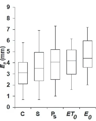
Ep of C ranged from 0.7 to 5.8 mm day^–1 on July 12 with a seasonal average of 3.03±1.23 (Fig. 3). Ep of S ranged from 0.7 to 6.9 mm day^–1 on July 5 with a seasonal average of 3.65±1.51. In the pan with macrophytes, Ep ranged from 1 to 7.3 mm day^–1 on August 6 with a seasonal average of 3.84±1.57. Reference Eo

and ETo values exceeded the measured Ep ones. Daily mean Eo and ETo were 4.65±1.43 and 3.93±1.25, respectively. The maximum Eo and ETo values occurred on June 25 and 28 as 7.2 mm day^–1and 6.1 mm day^–1, respectively.The probably reason of low pan Ep might has been the special geographical position of

April May June July August September i-season

2016 dry wet normal wet wet dry wet

Keszthely meteorological station. The meteorological station is placed at about 200 m from Keszthely Bay (Balaton Lake), that is sheltered by surrounded mountains causing lower wind speeds (Anda et al., 2016). In accordance with the studies of McVicar et al. (2012), there has also been a decline in near surface u, contributing to a reduced rate of evaporative demand.

Fig. 3. Statistical analysis for daily Class A pan evaporation, Ep during the 2016 growing season. The bottom and top of boxes are the 25th and 75th percentiles (the lower and upper quartiles), respectively, and the band near the middle of the boxes is the median (50th percentile). Vertical lines that end in a horizontal stroke above and below each box are drawn from the upper and lower hinges to the upper and lower adjacent values. C, S, and Ps denote Class A pan, Class A pan with sediment-covered bottom, and Class A pan implemented with macrophytes, respectively.

Both sediment cover and macrophytes placed Class A pan increased daily Ep

rates significantly. Increments in seasonal mean daily Ep rates were 16.3%

(p≤0.0001) and 23.8% (p≤0.0001) in S and Ps, respectively. Difference in measured daily mean Ep and computed Eo was even greater (42.3%; p≤0.0001).

No deviation between ETo and Ep of Ps (p≤0.2838) was observed, confirming that Class A pan Ep implemented with submerged macrophytes is closer to the computed reference ETo than that of the empty Class A pan. Surprising result emerged when Eo and ETo were compared; a 16.6% (P≤0.0001) overestimation was found with Eo in comparison to ETo.

According to daily mean Ep rates, the cumulative Ep values were 363.1, 427.7, and 461.5 mm in C, S, and Ps, respectively (Fig. 4). At the same time, higher reference E values were computed (Eo: 551.9 mm; ETo: 472.1 mm). The impact of pan implementation for total Ep was always highly significant (p≤0.0001). There was no difference in the measured cumulative Ep of Ps (461.5 mm) and computed Penman-Monteith ETo (472.1 mm) during the season of 2016 (p≤0.2400).

Fig. 4. Cumulative evaporations [mm] of Class A pan, implemented pan with macrophytes (Ps), and implemented pan with sediment cover (S), and the reference evaporation, Eo. ETo

denotes the Penman-Monteith reference evapotranspiration total.

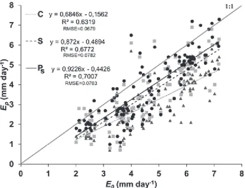
Irrespective of pan treatments, there was a large scatter in the data of daily measured Ep rates and computed reference Eo values (Fig. 5).

The slopes of linear regression between measured and computed E rates ranged from 0.68 to 0.92 (RMSE: 0.0679 – 0.7007 mm day^–1). Better fit was observed between Eo and Ep with implemented macrophytes (slope: 0.92).

Irrespective of pan treatments, computed Eo rates overestimated the measured Ep

values during the 2016 growing season.

The relationship between the measured Ep of implemented Class A pan and reference ETo (using Suttleworth formula) is improved in comparison to the relation between Ep and Eo.(Fig. 6).

Fig. 5. Relationship between the daily measured Class A pan evaporations (Ep) and daily reference evaporations (Eo) computed by the Suttleworth formula. C, S, and Ps denotes empty, sediment covered, and macrophyte implemented Class A pans, respectively.

Fig. 6. Relationship between the daily measured pan evaporation (Ep) of Class A pan implemented with macrophytes and daily reference evapotrationspiration (ETo) computed by Penman-Monteith (FAO-56) formula.

The slope of linear regression was close to 1 (1.03; RMSE: 0.0813 mm day^–1) implying that Penman-Monteith approximation (reference ETo) seems to be useful in estimation of the vaporation of the lake that contains submerged aquatic macrophytes.

3.3. Pan coefficient, K for implemented Class A pans

The ratio between the implemented Class A pan’s Ep and empty pan’s Ep provided a pan coefficient for those pan containing sediments (Ks) and/or macrophytes (Kp).

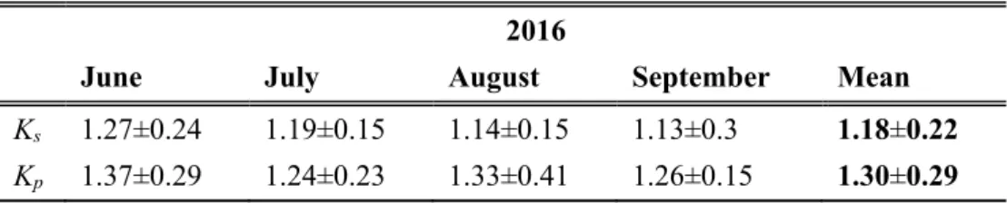
The way of obtaining these coefficients was similar to computing the widely applied crop coefficients (Kc) in evapotranspiration estimation. In accordance to increased daily and total Ep values for implemented Class A pans, the monthly average K values permanently exceeded 1 (Table 2). The seasonal mean Ks and Kp values were 1.18 (range: 1.13–1.27) and 1.30 (range: 1.24–1.37) in S and Ps, respectively. The highest increments in K values were observed during June, due to warmer weather conditions.

These K values may be useful in improving the Class A pan based E estimation of lakes or reservoirs which contain sediment covered bottom and/or submerged macrophytes.

Table 2. Monthly average pan coefficients for Class A pan with sediment-covered bottom (Ks) and containing macrophytes (Kp) in the growing season of 2016

2016

June July August September Mean

Ks 1.27±0.24 1.19±0.15 1.14±0.15 1.13±0.3 1.18±0.22 Kp 1.37±0.29 1.24±0.23 1.33±0.41 1.26±0.15 1.30±0.29

3.4. Impact of weather on Ep of implemented Class A pans

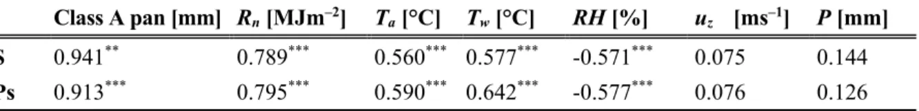
Correlation analysis to study the influence of weather variables (daily mean of Ta; daily means of water temperature, Tw; net radiation, Rn; relative humidity, RH;

wind speed u; precipitation P) on daily measured Ep rate of Class A pan with macrophytes and/or sediment cover was carried out (Table 3).

Table 3. Correlation coefficients (r) for daily measured evaporation rate (Ep) for Class A pans with macrophytes and/or sediment cover. The following daily weather variables were accounted: daily mean of air temperatures, Ta; daily means of water temperature, Tw; net radiation, Rn; relative humidity, RH; wind speed, uz; and precipitation, P

The closest relationship between the Ep of Class A pan and Ep of S (r=0.941) and Ps (r=0.913) was not unexpected. Meteorological variables related to available energy (Rn, Ta, Tw) have also high positive correlation coefficients in both implemented pan treatments (S and Ps). Rn had governmental role in Ep

regulation on the basis of its correlation coefficient size among energy related variables (r=0.789 and r=0.795 in S and Ps). Somewhat lower correlation coefficients of Ta and Tw ranged from r=0.56 (S) to r=0.642 (Ps). Martinez et al.

(2006) and McVicar et al. (2007) communicated the decisive effect of Tw on the rate of Class A pan Ep. Gundalia and Mrugen (2013) and Xiaomang et al. (2011) also found high positive correlation between Ta and Ep. In our study, a negative correlation of r= –0.57 was noticed with RH (both Ep of S and Ps), in accordance with earlier observations of Singh et al., (1992).

A weak positive correlation coefficient for u has not confirmed the earlier result of McVicar et al. (2012) for Ep. The probably reason of very loose relation between u and Ep may be the geographical position of Keszthely Bay, that is sheltered by Keszthely Mountains from the side of prevailing northern wind direction. Weak correlation of P with Ep came as no surprise, due to the water replacement practice of pan operation.

Ep rate is defined as the difference in vapor pressure between the pan’s surface and surrounding atmosphere, providing a simple integrated measurement of complex meteorological interaction between Rn, Ta, RH, uz, and Ep (Roderick et al., 2009). Due to strong variability in the magnitude of the above specified meteorological elements, measured Ep rates can strongly differ from place to place (Yang and Yang, 2012). These qualifying differences in spatial Ep might also be displayed in variation of correlation coefficients existing between meteorological variables and Ep rates.

Only easily accessible meteorological variables are included in the multiple stepwise regression analysis (Ta, RH, uz, P). Class A pan, Rn and Tw were excluded

Class A pan [mm] Rn [MJm^–2] Ta [°C] Tw [°C] RH [%] uz [ms^–1] P [mm]

S 0.941^** 0.789^*** 0.560^*** 0.577^*** -0.571^*** 0.075 0.144 Ps 0.913^*** 0.795^*** 0.590^*** 0.642^*** -0.577^*** 0.076 0.126

* Marginally significant correlation |r|>0.1, p<0.01

** Marginally significant correlation |r|>0.1, p<0.001

*** Significant correlation |r|>0.4, p<0.0001

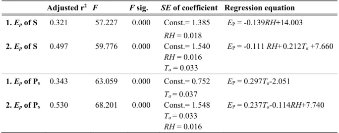
from the investigation. In the course, three meteorological variables remained in the regression equations (Ta, uz, and RH). These meteorological variables are available even in such places where meteorological stations are missing (research stations, universities, etc.). Our analysis showed that two meteorological variables (Ta and RH) impacted the Ep of Ps and S the most (Table 4). The first two equations of Table 4 present the possibility of computing E of a lake/reservoir with macrophytes and/or sediments, when the only available meteorological variable is the Ta (in Ps) or RH (in S). The second two equations of E, estimation when macrophytes and sediment cover are accounted, contain two meteorological variables, Ta and RH. Observation of Ta or RH might not cause difficulties in the present time.

Table 4. Multiple stepwise regression analysis between meteorological elements (air temperature, Ta; relative humidity, RH; wind speed uz,, precipitation, P) and measured Class A pan evaporation (Ep) with macrophytes (PS) and sediment covered bottom (S) in the season of 2016. r: coefficient of multiple correlation.

3.5. Simple water budget terms on Balaton Lake (Keszthely Bay) during the growing season of 2016

There are two important terms describing the simplified water budget of a lake:

the precipitation P as an input and the evaporation E as the output of water.

Specification of exact water balance of studied site was excluded from our investigation. Our purpose was a simple comparison of the two most important simplified water balance members at Keszthely Bay. The area of Keszthely Bay is 39 km², less than 10% of the whole area of Balaton Lake. Based on local observations, the submerged macrophytes occupies 5–10% of the whole bay (Anda et al., 2016). The remaining part of the bay accounted for as covered bottom with sediments.

Adjusted r² F F sig. SE of coefficient Regression equation 1. Ep of S 0.321 57.227 0.000 Const.= 1.385

RH = 0.018

EP = -0.139RH+14.003 2. Ep of S 0.497 59.776 0.000 Const.= 1.540

RH = 0.016 Ta = 0.033

EP = -0.111 RH+0.212Ta +7.660

1. Ep of Ps 0.343 63.059 0.000 Const.= 0.752 Ta = 0.037

EP = 0.297Ta-2.051 2. Ep of Ps 0.530 68.201 0.000 Const.= 1.548

Ta = 0.033 RH = 0.016

EP = 0.237Ta-0.114RH+7.740

Despite wet conditions of the growing season, computed E of Keszthely Bay surpassed seasonal amount of P in 2016 (Table 5). Slightly more than 90% of E derived from P in the 2016 growing season. On daily mean basis, the E rate of Keszthely Bay increased with 16.9% when macrophytes and sediment cover were accounted. Increment in seasonal total E for the whole bay resulted 264,000,000 m³ water, when macrophytes and sediment cover were included in Keszthely Bay’s E estimation. During arid seasons, this E rate may increase substantially strengthening the importance of E related investigations of natural lakes.

Table 5. Seasonal sums of precipitation (P) and evaporation (E) [mm] of Keszthely Bay including daily E rates [mm day^–1]. The E estimates of the lake were based on weighting averages of a) using pan coefficients with sediment-covered bottom (Ks), and macrophytes (Kp) and b) simple Class A pan measurements.

4. Conclusions

A simple approach was presented to evaluate the E of a natural fresh water lake in Hungary. To achieve this goal, Class A pans were implemented with aquatic submerged macrophytes and/or their bottom was covered by sediment. Ep rate of treated Class A pans increased significantly. The impact of macrophytes and sediment cover on the E of the lake can be computed directly through using pan’s coefficients.

In our study, we received a Class A pan coefficient of above 1 (Kas:1.18;

Kap:1.3) in comparison to the calculated potential evapotranspiration, which is in contrast to the most reported cases in the literature, where values of well below 1 (around 0.75) were received. Similarly to our outstanding results in 2016, annual

a) Simple water budget terms of Keszthely Bay (macrophytes and sediment cover included) Seasonal sums Daily rates Water total

[mm] [mm day^–1] [10⁶ m³]

P E Δ E P E Δ

328.5 430.69 –102.19 3.59 12.81 16.8 –3.99

b) Simple water budget computed by Class A pan data only

Seasonal sums Daily rates Water total

[mm] [mm day^–1] [10⁶ m³]

P Ep Δ Ep P Ep Δ

328.5 363.15 –34.65 3.03 12.81 14.16 –1.35

mean value of 0.99 for one separate warm and arid year was published by Sabziparvar et al. (2009). Allen et al. (1998) have also imparted that Class A pan coefficient may vary highly depending on the geographical site and the actual weather conditions.

The reason of Kc deviation could lie in biased wind profile – i.e., biased measurement of wind speed and/or its correction to 2 m height. Moreover, the special hill-surrounded (shadowed) location of Keszthely Agrometeorological Research Station may also reduce the impact of wind on evaporation. Roderick et al. (2007) revealed differences among 41 investigated sites between 1977 and 2004, where decreasing wind speed was found to be the main reason for changing Class A pan evaporation. Other possible reason of altered Kc may be the estimation of net radiation instead of measurement together with neglected factors influencing pan energy balance. Therefore, our Class A pan coefficient should be used with attention to local environmental conditions, and should be re-calibrated before application, if possible.

Growing season of investigation has the characteristic of a wet weather. Even in the course of the wet season, the increment in E of Keszthely Bay (Balaton Lake) reached 16.9% (264,000,000 m³), when macrophytes and sediments were also accounted. This simple approach using pan coefficients may extend the accuracy of the E estimation of natural lakes, based on Class A pan in a broader circle than earlier.

Acknowledgement: We acknowledge the financial support of Széchenyi 2020 under the EFOP-3.6.1- 16-2016-00015. The project is co-financed by Széchenyi 2020.

References

Allen, R.G., Clemmens, A.J., Burt, C.M., Solomon, K., and O'Halloran, T., 2005: Prediction accuracy for projectwide evapotranspiration using crop coefficients and reference evapotranspiration. J. Irrig. Drain. Eng. ASCE, 131, 24–36.

https://doi.org/10.1061/(ASCE)0733-9437(2005)131:1(24)

Allen, R.G., Pereira, L.S., Raes, D., and Smith, M., 1998: Crop evapotranspiration – guidelines for computing crop water requirements. FAO Irrigation and Drainage Paper 56, Rome, Italy.

Anda, A., Simon, B., Soos, G., Teixeira da Silva, J.A., and Kucserka, T., 2016: Effect of submerged, freshwater aquatic macrohytes and littoral sediments on pan evaporation in the Lake Balaton region, Hungary. J. Hydrol. 542, 615–626.

https://doi.org/10.1016/j.jhydrol.2016.09.034

Anda, A., Teixeira da Silva, J.A., and Soos, G., 2014: Evapotranspiration and crop coefficient of the common reed at the surroundings of Lake Balaton, Hungary. Aquatic Bot. 116, 53–

59. https://doi.org/10.1016/j.aquabot.2014.01.008

Barrat-Segretain, H.M., 1996: Strategies of reproduction, dispersion, and competition in river plants: A review. Vegetatio 123, 13–37.https://doi.org/10.1007/BF00044885

Brothers, S., Hilt, S., Meyer, S., and Köhler, J., 2013: Plant community structure determines primary productivity in shallow, eutrophic lakes. Freshw. Biol. 58, 2264–2276.

https://doi.org/10.1111/fwb.12207

Gundalia, M.J., and Mrugen D.B., 2013: Modelling pan evaporation using mean air temperature and mean pan evaporation relationship in middle south Saurashtra Region.

A review. Int. J. Water Res. Environ. Engin. 5, 622–629.

Hilt, S., Adrian, R., Köhler, J., Monaghan, M.T., and Sayer, C., 2013: Clear, crashing, turbid and back e long-term macrophyte changes in a shallow lake. Freshw. Biol. 58, 2027–

2036. https://doi.org/10.1111/fwb.12188

Jacobs, A.F.G., Heusinkveld, B.G., and Lucassen, D.C., 1998. Temperature variation in a class A evaporation pan. J. Hydrol. 206, 75–83. https://doi.org/10.1016/S0022-1694(98)00087-0 Kim, S., Shiri, J., Singh, V.P., Kisi, O., and Landeras, G., 2015: Predicting daily pan evaporation

by soft computing models with limited climatic data. Hydrol. Sci. J. 60, 1120–1136.

https://doi.org/10.1080/02626667.2014.945937

Lim, W.H., Roderick, M.L., Hobbins, M.T., Wong, S.C., and Farquhar, G.D., 2013: The energy balance of a US Class A evaporation pan. Agric. Forest Meteorol. 182–183, 314–331.

https://doi.org/10.1016/j.agrformet.2013.07.001

Linacre, E.T., 1994: Estimating United States Class-A pan evaporation from few climate data.

Water Int. 19, 5–14. https://doi.org/10.1080/02508069408686189

Majidi, M., Alizadeh, A., Farid, A., and Vazifedoust, M., 2015: Estimating evaporation from lakes and reservoirs under limited data condition in a semi-arid region. Water Res.

Manage, 29, 3711–3733. https://doi.org/10.1007/s11269-015-1025-8

Martí, P., González-Altozano, P., López-Urrea, R., Mancha, L.A., and Shiri, J., 2015: Modeling reference evapotranspiration with calculated targets. Assessment and implications. Agric.

Water Manage. 149, 81–90. https://doi.org/10.1016/j.agwat.2014.10.028

Martinez, J.M.M., Alvarez, V.M., Gonzalez-Real, M.M., and Baille, A., 2006: A simulation model for predicting hourly pan evaporation from meteorological data. J. Hydrol. 318, 250–261. https://doi.org/10.1016/j.jhydrol.2005.06.016

McVicar, T.R., Roderick, M.L., Donohue, R.J., Li, L.T., Van Niel, T.G., Thomas, A.,Grieser, J., Jhajharia, D., Himri, Y., Mahowald, N.M., Mescherskaya, A.V., Kruger,A.C., Rehman, S., and Dinpashoh, Y., 2012: Global review and synthesis of trends in observed terrestrial near-surface wind speeds: implications for evaporation. J.Hydrol. 416–417, 182–205.

https://doi.org/10.1016/j.jhydrol.2011.10.024

McVicar, T.R., Van Niel, T.G., Li, L.T., Hutchinson, M.F., Mu, X.M., and Liu, Z.H., 2007:

Spatially distributing monthly reference evapotranspiration and panevaporation considering topographic influences. J. Hydrol. 338, 196–220.

https://doi.org/10.1016/j.jhydrol.2007.02.018

Monteith, J.L., 1965: Evaporation and environment. In (Ed.: Fogg, G.E.) The State and Movement of Water in Living Organism. Proc. XIX. Symp. Soc. Exp. Biol. Cambridge University Press, Cambridge. 205–234.

Penman, H.L., 1948: Natural evaporation from open water, bare soil and grass. Proc. Royal Soc. London. Ser. A, Mathematical Phys. Sci. 193 (1032), 120–145.

https://doi.org/10.1098/rspa.1948.0037

Roderick, M.L., Rotstayn, L.D., Farquhar, G.D., and Hobbins, M.T., 2007: On the attribution of changing pan evaporation. Geophys. Res. Lett. 34, L17403.

https://doi.org/10.1029/2007GL031166

Rotstayn, L.D., Roderick, M.L., and Farquhar, G.D., 2006. A simple pan-evaporation model for analysis of climate simulations: evaluation over Australia. Geophys. Res. Lett. 33, L17715. https://doi.org/10.1029/2006GL027114

Sabziparvar, A.A., Tabari, H., Aeini, A., and Ghafouri, M., 2010: Evaluation of Class A Pan Coefficient Models for Estimation of Reference Crop Evapotranspiration in Cold Semi- Arid and Warm Arid Climates. Water Res. Manage 24, 909–920.

https://doi.org/10.1007/s11269-009-9478-2

Shiri, J., Dierickx, W., Baba, A.P.A., Neamati, S., and Ghorbani, M.A., 2011: Estimating daily pan evaporation from climatic data of the State of Illinois, USA using adaptive neuro- fuzzy inference system (ANFIS) and artificial neural network (ANN). Hydrol. Res. 42, 491–502. https://doi.org/10.2166/nh.2011.020

Shuttleworth, W.J., 1993. Evaporation. In (ed.: Maidment, D.R.) Handbook of Hydrology.

McGraw and Hill, New York.

Singh, R., Bishnoi, O.P., and Ram, N., 1992: Relationship between evaporation from class 'A' open pan evaporimeter and meteorological parameters at Hisar. Haryana Agri. Univ. J.

Res. 22, 97–98.

Soos, G. and Anda, A., 2014: A methodological study on local application of the FAO-56 Penman- Monteith reference evapotranspiration equation. Georgikon for Agric. 18, 71–85.

SPSS Statistics version 17.0 software. IBM Corp., New York, USA.

Vári, Á., 2012. Propagation and growth of submerged Macrophytes in Lake Balaton. PhD Dissertation.

Wang, L., Kisi, O., and Zounemat-Kermani, Li, H., 2017: Pan evaporation modeling using six different heuristic computing methods in different climates of China. J Hydrol.

544, 407–427. https://doi.org/10.1016/j.jhydrol.2016.11.059

WMO Report, 1975. Drought and Agriculture. WMO Techn. Note No. 138.

Xiaomang, L., Yuzhou, L., Dan, Z., Minghua, Z., and Changming, L., 2011. Recent changes in pan-evaporation dynamics in China. Geophys. Res. Lett. 38, 13–19.