DOI:10.28974/idojaras.2020.1.1
IDŐJÁRÁS
Quarterly Journal of the Hungarian Meteorological Service Vol. 124, No. 1, January – March, 2020, pp. 1–23
Impact of the stratosphere on the sea surface temperature and ENSO based on HadGEM control runs comparing
high top and low top model configurations
Shaomin Cai1,2, Weijia Zhang*,1,3, and Yizhou Zhao4
1 Department of Math&Physics, Shaoxing University No.508, Huancheng West Road, Shaoxing 312000, China
2Department of AOP Physics, University of Oxford Wellington Square, Oxford OX1 2JD, United Kingdom
3 Visiting Scholar, Department of AOP Physics, University of Oxford Wellington Square, Oxford OX1 2JD, United Kingdom
4 Department of Astronautics, Nanjing University of Aeronautics and Astronautics No. 169, Sheng Tai West Road, Nanjing 211106, China
Corresponding Author e-mail: zhangw@physics.ox.ac.uk (Manuscript received in final form April 16, 2019)
Abstract⎯ Numerous studies on the effects of the El Niño-Southern Oscillation (ENSO) on the stratosphere have been conducted in recent years. However, few of these have examined whether the use of an adequate representation of the stratosphere might affect simulations of the ENSO. In the present work, sea surface temperature data from two numerical model configurations, namely one with a well-resolved stratosphere, the “high top configuration”
(Hadley Centre Global Environmental Model, HadGEM2-CCS), and the other without a well- resolved stratosphere, the “low top configuration” (HadGEM2-CC), are employed to study the impact of the stratosphere on the surface climate, especially on the ENSO. A pre-industrial control run is performed to eliminate interference from other factors, such as greenhouse gas warming and volcanic eruptions. Based on the present research, both model configurations function reasonably well and have shown little difference from each other when analyzng the global annual and seasonal mean sea surface temperatures, except for the Northern Atlantic Ocean region. A statistical analysis performed using the t-test method shows that the significant differences in the annual and seasonal mean sea surface temperatures in the Northern Atlantic region result from real signals rather than random noises. Furthermore, the configuration with a better representation of the stratosphere simulates the quasi-period of the ENSO and the seasonal phase-locking characteristics of El Niño more precisely. Therefore, it is probably advantageous to adopt climate models that resolved stratosphere for a more realistic representation of ENSO climatology and its possible variations under certain conditions.
Key-words:stratosphere, sea surface temperature, ENSO, HadGEM, high top configuration, low top configuration
1. Introduction
The present work aims to determine the effects of the stratosphere on global climate as well as on the El Niño-Southern Oscillation (ENSO) by examining and comparing numerical simulations both with and without a well-resolved stratosphere.
1.1. The ENSO phenomenon
The ENSO is a quasi-periodic climate phenomenon that occurs in the tropical Pacific and is attributed to a coupled ocean-atmosphere interaction.
The atmospheric aspect, called the Southern Oscillation, was first identified by Walker (1923, 1924) as a seesaw of surface pressure between the central tropical Pacific and the Indonesian Archipelago. The three-dimensional circulation pattern explaining Southern Oscillation was described by Bjerknes (1969) and designated as the ‘Walker Circulation’ (Fig. 1). The quasi-periodic warming of the waters off the coast of Peru and Ecuador is called El Niño. El Niño has long been understood to be part of an oceanic oscillation that extends westward along the equator. Bjerknes (1966, 1969) was among the first to recognize its connection to the Southern Oscillation.
Fig. 1. Schematic diagrams of (a) normal conditions and (b) El Niño conditions in the Pacific Ocean. Fromwww.pmel.noaa.gov/tao/elnino/ninonormal.html
During normal years, as shown in Fig. 1(a), a particularly strong cooling in the eastern Pacific is called La Niña. Under El Niño conditions, as shown in Fig. 1(b), the Walker circulation reverses, resulting in El Niño events. El Niño
followed by neutral conditions. However, El Niño events have a typical life cycle that tends to be phase-locked with the seasonal cycle, with warm SST anomalies tending to appear in January, strengthening during the year, and eventually peaking in the northern winter one year after their onset (Wang, 1995). This seasonal phase locking is also observed in the climate model results examined here (see Section 3.2). Although ENSO events are irregular, in the historical record, the length of this interval has varied from 2 to 7 years (NOAA Climate Prediction Centre (2005-12-19)).
The ENSO is widely accepted to be the largest source of internal variability in the global climate system (Trenberth et al., 1998). The eastward displacement of the atmospheric heat source overlying the warmest water results in significant changes in the global atmospheric circulation, which forces weather changes in regions remote from the tropical Pacific. These remote influences are known as teleconnections.
1.2. ENSO and the stratosphere
El Niño events are associated with maximum warm anomalies occurring in the tropical Pacific. Thus, it is useful to study these events by simulating aspects of surface climate. Observational and modeling studies over the past two decades have fundamentally changed our understanding of the role of the stratosphere in surface weather and climate. Interactions between the stratosphere and other components of the earth’s system, from the troposphere to the deep ocean and possibly even the ice sheets of Greenland and Antarctica, reveal coupling across a wide range of spatial and temporal scales. In response to these discoveries, operational forecasts, seasonal predictions, and coupled climate models are raising their lids by adding model layers, incorporating additional stratospheric processes and assimilating data higher into the stratosphere than ever before (Gerber et al., 2012).
Van Loon and Labitzke (1987) studied the statistical relationship between ENSO and the Arctic stratosphere. They found that strong El Niño events are associated with a strong Aleutian High and weak polar vortex in the stratosphere.
Furthermore, the stratosphere appears to play an important role in transmitting the tropical ENSO signals to the mid-latitudes (e.g., Bell et al., 2009). Extra tropical upward wave propagation intensified during warm ENSO events in the boreal winter, modulating the meridional overturning circulation of the stratosphere and the stratospheric polar vortex (Garcia-Herrera et al., 2006). The vortex anomalies, ultimately, then propagated downward, affecting the mid-latitudes in the troposphere (Cagnazzo and Manzini, 2009).
Several modeling studies have shown that including a well-resolved stratosphere could produce more reliable tropospheric climate change projections.
For example, Hardiman et al. (2012) suggested that simulations should be performed using stratosphere-resolving general circulation models to capture the
influence of teleconnections and stratospheric processes on surface climate. This finding also indicates that little distinction is found between the model simulations with and without a well-resolved stratosphere, unless the effects of teleconnections on the surface fields during specific years are considered (e.g., the ENSO on the northern extra tropical mean sea level pressure (MSLP)).
However, most of the studies included the influences of various possible factors interfering with the interconnectedness of the ENSO and the stratosphere, such as seasonality and nonlinearity (Van Loon and Labitzke, 1987; Manzini et al., 2006), volcanic eruptions (Labitzke and Van Loon, 1989) and ozone depletion (Kiehl and Boville, 1988). However, these observational analyses may benefit from further comparisons with control run simulations. Control run simulations allow for the systematic study of the possible influences by excluding external factors, and they only differ in the stratosphere representations.
Therefore, to study the dynamical impact of the stratosphere alone on the surface climate, and the ENSO in particular, the present work used numerical simulations from model configurations with and without a well-resolved stratosphere. These model configurations are the two configurations of the Hadley Centre Global Environmental Model (HadGEM) run at the Met Office Unified Model for CMIP5. (Refer to Section 2 for more details.) Pre-industrial control runs were used to investigate the effects of the vertical height and resolution of the stratosphere alone on surface climate, and again, the ENSO in particular.
(Details of the control run are described in the Section 2.)
In the present work, the first aspect under review is the annual and seasonal mean SSTs in both model configurations, which are compared with observations.
The effects of random variability on the annual mean SSTs are also examined.
The second aspect under review focuses on the equatorial tropical region in both model configurations to investigate the quasi-period of ENSO events through a power spectrum. The third aspect is the study of the evolution of the ENSO in both model configurations through Hovmoller diagrams. (Details are shown in Section 3.4.) A detailed analysis of the possible factors that may give rise to the differences in the ENSO characteristics between the configurations, as described in Section 3, will be the subject of a later and more extensive study, but these are discussed in general terms at the end of this report.
2. Models and methods
Two configurations of the HadGEM run at the Met Office Unified Model for CMIP5 are used in the present work. These two configurations are the HadGEM2-CCS (high top configuration) and HadGEM2-CC (low top configuration) (Martin et al., 2011), which differ only in their vertical extent and vertical resolution. The high top configuration includes a well-resolved stratosphere, incorporating 60 vertical levels (L60) and an upper boundary at 85 km (mesopause). The low top configuration has
38 vertical levels (L38) and an upper boundary at 40 km (mid stratosphere). As shown in Appendix 1, the vertical resolutions show the details of how these levels are defined. The high top configuration is better by more than a factor of two in the vertical resolution within the stratosphere (Collins et al., 2008).
To obtain a clear view of the dynamic impact of the vertical height and resolution of the stratosphere alone on the ENSO, the ‘control runs’ of both the high top and the low top configurations were used instead of the historical runs, as performed in Hardiman et al. (2012). The control run is a simulation using pre- industrial levels of CO2 and ozone that are held constant with time (Taylor et al., 2009). In other words, the influence of volcanic eruptions and increasing CO2
concentrations is eliminated. The pre-industrial control run also serves as the baseline for the analysis of historical and future scenarios, because it runs with non-evolving, pre-industrial conditions. The pre-industrial control run is used in addition to estimate the unforced variability of the model (Taylor et al., 2009).
Therefore, the two sets of SST data in this work result from the pre-industrial control runs of the high top and low top configurations, which are publicly available from CMIP5 data centers and were downloaded by a DPhil student. The present research is based on these two sets of SST data. The SSTs used in the present work are determined by four variables: time, longitude, latitude, and depth. The depth is set to one meter below the ocean surface, which is sufficient to represent surface temperature variability. The time (t) unit is one month, which means the SST is a monthly average temperature. Both configurations were run over the same period of time, spanning 240 years (t=2880) in total. However, because some of the data are missing in the SST data sets of both configurations (details in the Appendix 2), only 150 years of data were used for the analysis, which is still sufficiently long to study quasi-periodic events such as the ENSO.
Hence, adequate realizations for examining its statistics are available.
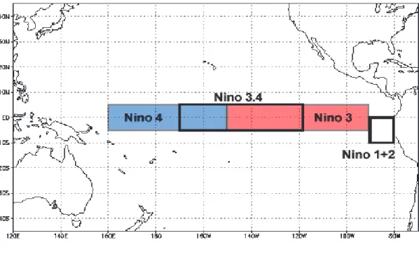
There are different ways of measuring the strength of the ENSO (Trenberth 1997). For the oceanic component, the most common method is to average the SST anomalies over certain regions termed Niño 1+2, Niño 3, Niño 4, and Niño 3.4 (Fig. 2). These SST-based indices are statistically positive for El Niño and negative for La Niña. In addition, there are various procedures to evaluate the SST anomalies. This study adopted two of these: one as SST anomalies with the seasonal cycle and the other without. The SST anomalies evaluated with the seasonal cycle computed by subtracting the annual mean SST from each SST, while those without the seasonal cycle are determined by subtracting the monthly average of the corresponding month (relevant Matlab codes are listed in Appendix 5).
Fig. 2. Niño regions (www1.ncdc.noaa. gov/pub/data/cmb/teleconnections/nino- regions.gif)
El Niño events are then defined based on the conditions of certain thresholds being exceeded. The present work utilized the official National Oceanic and Atmospheric Administration (NOAA) definition stating that El Niño (La Niña) is a phenomenon in the equatorial Pacific Ocean characterized by five consecutive, three-month running-means of SST anomalies in the Niño 3.4 region above (below) the threshold of +0.5 0C (-0.5 0C). This standard measurement is known as the Oceanic Niño Index (ONI) (refer to NOAA ONI in the references for details).
In this work, the eastern and central equatorial Pacific Ocean regions, Niño3 (5S–5N, 90W–150W) and Niño 3.4 (5S5N, 120W–170W), were used to measure the strength of ENSO and ONI of Niño3.4. Moreover, to determine how well the SST was simulated in both model configurations, corresponding plots from NOAA were used for comparison.
3. Results and analysis
Using the high top simulations run with the Met Office Unified Model for CMIP5, and equivalent low top simulations, the present work studies the effects of the inclusion of a well-resolved stratosphere through general circulation model climate simulations of oceanic surface climate.
3.1. Global annual climatology
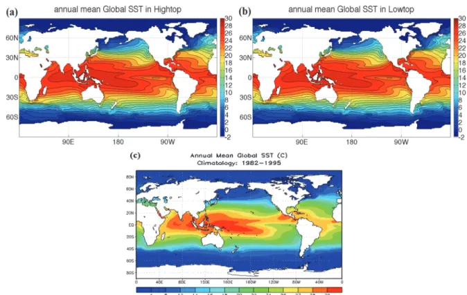
Figs. 3(a) and (b) show the climatology plots of global SST averaged over 150 years of control data for the high top and low top configurations, respectively, and (c) shows the observed annual mean sea surface temperature climatology from the National Oceanic and Atmospheric Administration (NOAA, http://www.cpc.ncep.noaa.gov/ products/precip/CWlink/climatology/). Both high top and low top configurations generally captured the warmest mean temperature, which occurs near 120° E in the tropics and the coldest around the North and South Poles. The findings agree well with plot (c), which also shows a cold tongue in the east Pacific Ocean along the coastline of South America.
Fig. 3. Global sea surface temperature averaged over 150 years; (a) the high top model configuration, (b) the low top model configuration, and (c) the annual mean of global SST from 1982 to 1995, plot from the NOAA National Weather Service.
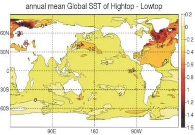
Fig. 4 shows the annual mean global SSTs of the high top run minus the low top run, i.e., the difference between Figs. 3(a) and (b). The differences in temperature are less than 1 0C between the high top and low top model configurations, except in the northern extra-tropical region. The significant differences in the northern Atlantic region may be attributed to various causes, including the ocean circulation or different surface winds. All these possible
reasons result from the differences between the high top and low top configurations’ parameters, which are different in the vertical extension and vertical resolution of the stratosphere.
Fig. 4. Differences in the annual mean global SSTs between the high top and low top model configurations.
The present work then further examined whether the differences are attributable to noise or real signal differences between the high top and low top configurations. Thus, it is necessary to consider a steady state configuration. The first 20 (out of 240 available) years of data were disregarded to cut off the spinning up processes. However, noise still remains because of the random variability. To test whether the high top and low top annual SSTs are significantly different, a standard 2-sample t-test is introduced.
The t-test is the most commonly used method to evaluate the differences in the means between two samples with normal distributions (http://www.statsoft.com/ textbook/basic-statistics/). The t-value is determined as:
, (1)
1 2
1 2
2
X X
X X
t
S n
= −
×
, (2)
where and are the means of data sets 1 and 2, respectively. S×1×2 is the standard deviation of the combined data, defined by Eq.(2). n is the number of data points in each data set, which refers to the number of time points here (81885 points). In Matlab, the function h = ttest2(x,y) was used in this study.
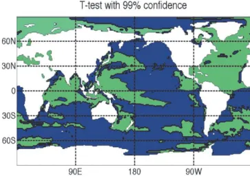
The data were also tested for normality 1 similar variance to ensure the t-test was valid. In Fig. 5, the green area indicates that h=1 and blue indicates that h=0.
This means that differences between the annual mean SSTs of the high top and low top model configurations in the green area result from real signal differences between the high top and low top runs at a 99% confidence level. In contrast, the possibility that the differences in the blue area are generated by noise cannot be disregarded. In the northern Atlantic Ocean region, the differences in annual mean temperature between the high top and low top model configurations are mainly statistically significant with 99% confidence. The SSTs in the high top configuration in this region are expected to have more variability as SST is more influenced by the stratosphere (Baldwin and Dunkerton, 2001).
Fig. 5. t-test of the high top and low top annual mean global SSTs.
2 2
1 2 1 2
1( )
X X 2 X X
S = S +S
X1 X 2
3.2. Global seasonal climatology
The seasonal mean climatology plots (Fig. 6) from high top and low top configurations and those from the NOAA National Centres for Environment and Predictions (NCEP) reanalysis are reported. The NOAA NCEP reanalysis data set is a continually updated grided data set representing the state of the Earth’s atmosphere, incorporating observations and numerical weather prediction (NWP) model outputs dating back to 1948. It could serve as observational data or data close to observations. The data set was adopted to create seasonal SST climatology plots for comparison. (The plots are available at www.esrl.noaa.gov/psd/cgibin/data/composites/printpage.pl)
In this research, spring is considered to begin on the first day of March, and each season lasts 3 months, which is generally the definition used in meteorology for the northern hemisphere. Therefore, spring begins on March 1, summer on June 1, autumn on September 1, and winter on December 1.
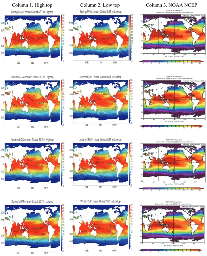
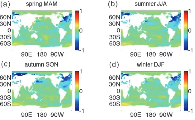
The corresponding seasonal climatology plots from both the high top and low top configurations were initially compared with those from the NCEP reanalysis (plots in column 3 of Fig. 6). Both the high top and low top configurations generally agree well with the observations. Fig. 7 shows the seasonal mean global SSTs for the high top minus the low top runs. The differences in temperature are less than 1 0C between the high top and low top configurations, except in the northern extra-tropical region, which is similar to the annual mean in Fig. 4. The t-test for these seasonal means was also computed, and the results show a pattern similar to the one in Fig. 5. The seasonal climatology is in reasonable agreement with the theory suggested in Baldwin and Dunkerton (2001).
Column 1. High top Column 2. Low top Column 3. NOAA NCEP
Fig. 6. Seasonal mean global sea surface temperature climatology plots from the high top configuration (column 1), the low top configuration (column 2), and the NOAA National Centres for Environment and Predictions (NCEP) reanalysis (column 3, available at http://www.esrl.noaa.gov/psd/cgi-bin/data/composites/printpage.pl). The first row represents spring (MAM), the second represents summer (JJA), the third row represents autumn (SON), and the last row represents winter (DJF).
Fig. 7. Differences in the seasonal mean global SSTs between the high top and low top configurations during (a) spring (MAM), (b) summer (JJA), (c) autumn (SON), and (d) winter (DJF).
3.3. ENSO power spectrum
After studying the global behavior, the focus now is exclusively on the behavior of El Niño as described by the SST variability in the equatorial central and eastern Pacific region, i.e., the Niño 3 and Niño 3.4 regions of both the high top and low top configurations. The normalized power spectra of the corresponding monthly SST anomalies are computed by taking the fast Fourier transform of a time series as the output in its frequency spectrum (based on the code from http://blinkdagger.com/matlab/matlab-introductory-fft-tutorial/).
Detailed Matlab codes are shown in Appendix 5.
First, the Niño indices were computed by averaging the SST anomalies over the corresponding Niño regions. For example, low Niño 3 indices without the seasonal cycle are computed by averaging the low top SST anomalies without the seasonal cycle over the Niño 3 region. The time series can then be plotted (Fig. 8), and the corresponding power spectra can then be computed (Fig. 9).
The power spectra of the low top Niño 3 indices with the seasonal cycle and those without the seasonal cycle are identical, except near the 1 year per cycle strong peak observed in that with the seasonal cycle. This finding indicates that the method adopted to remove the seasonal cycle is reasonable for investigating
the stratospheric impacts on ENSO quasi-periods. In addition, studying the differences without the representation of the seasonal cycle may be easier, because the effect of the seasonal cycle in power spectrum study can be eliminated. The horizontal axis represents the number of years per cycle over a total of 150 years, and a frequency band of 10 years per cycle is statistically more reliable than the rest. For example, a frequency of 10 years per cycle has 15 cycles as a sampling ensemble. Therefore, the focus was directed towards a range of 0 to 10 years per cycle on the Niño indices without the seasonal cycle.
The time series of the Niño 3 and Niño3.4 indices without the seasonal cycle for the both high top and low top configurations were produced (not shown here) as well as the corresponding power spectra (Figs. 10 and 11).
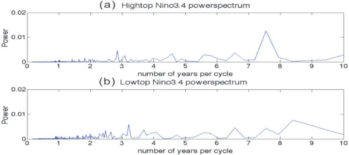
Both the high top Niño3 and Niño3.4 power spectra show peak bands over approximately 3 to 8 years per cycle, especially in the band of 7 to 8 years per cycle. The major ENSO events simulated in the low top configuration have quasi- periods of 7 to 8 years. Some of the ENSO events are located in a period band of 5 to 7 years, as well as a period of approximately 3 years. The low top power spectra also capture the peak band of 3 to 8 years per cycle. However, a stronger peak is observed in the region of 8 to 9 years per cycle. The major ENSO events simulated in the low top configuration have quasi-periods of 8 to 10 years. Only a few events have a quasi-period of approximately 6.5 years or 5.6 years.
By just considering the power spectra in Figs. 10 and 11, the high top configuration matches better with the general quasi-periods of the ENSO, which vary from 2 to 7 years. Most of the power is found within the band of 2 to 8 years for the high top configuration, whereas most of the power is found within the band of 9 to 10 years for the low top configuration. However, this conclusion is imprecise, thus requiring further study.
Fig. 8. The time series of the low top Niño 3 index: the SST anomalies without the seasonal cycle.
Fig. 9. Corresponding power spectra of time series in Fig. 8: the power spectrum without the seasonal cycle. The x-axis represents the number of years per cycle and the y-axis is the power.
Fig. 10. Power spectra of the Niño3 SST anomalies without the seasonal cycle for (a) the high top configuration and (b) the low top configuration.
Fig. 11. Power spectra of the Niño 3.4 SST anomalies without the seasonal cycle for (a) the high top configuration and (b) the low top configuration.
Using the NOAA definition described in Section 2 to classify the El Niño events, Appendix 3 shows the time series of both the high top and low top Niño 3.4 ONI with a threshold of 0.5 0C. The power spectra (not shown) corresponding to the time series are similar to those shown in Fig. 11. The time series are then used to classify El Niño episodes. The criterion, which is often used to classify El Niño episodes, is that five consecutive 3-month running mean SST anomalies exceed the threshold. A list of El Niño episodes from the high top configuration can then be produced (Matlab code is in Appendix 5). With this list, several examples of the evolutions of El Niño episodes can then be plotted.
3.4. ENSO evolutions
Changes in the SST anomalies shown above during the ENSO cycle are accompanied by wind anomalies that cause the mean easterlies to weaken during El Niño events and strengthen during La Niña events. To illustrate the structure of the evolution over time during ENSO events, both high top and low top equatorial SSTs are considered as a function of longitude and time (Figs. 12 and 13), and SST anomalies along the Equatorial Pacific are represented as a Hovmoller diagram for the high top and low top configurations, respectively. A Hovmoller diagram created from the NOAA Tropical Atmosphere and Ocean (TAO) project of the equatorial SST and SST anomalies from 1990 to 2000 is available in Appendix 4 for reference.
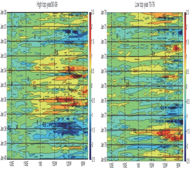
Fig. 12 shows the high top SST anomalies in the equatorial Pacific region averaged over the latitude band 5S to 5N, and Fig. 13 shows the low top configuration anomalies. A red color indicates a strong El Niño signal, and dark blue represents La Niña signals. A total of 15 diagrams were produced, covering 150 years each for the both high top and low top configurations. Each diagram covers a 10-year time scale (e.g., Fig. 12, years 30 to 39). Based on the high top configuration Hovmoller diagrams, the majority of El Niño events tend to reach their peak towards the end of the calendar year, such as the one shown in Fig. 12, in which the El Niño event reaches its maximum between December of year 36 and January of year 37. However, in the low top configuration diagrams, El Niño events do not show this seasonal phase-locking property. For example, the El Niño event between year 78 and year 79 shown in Fig. 13 peaks around summer.
The Hovmoller diagrams shown in this work for both high top and low top configurations contain relatively active ENSO phenomena, with El Niño events followed by La Niña events. Several other diagrams show neutral conditions (normal years) following El Niño or La Niña events. This finding is consistent with the general characteristics of the ENSO presented in the introduction.
Fig. 12. Hovmoller diagram from January in year 30 to January in year 40 of the high top configuration simulation. The horizontal axis is the longitude from 110E to 80W; the vertical axis is the time stating with January in year 40 and ending with January in year 30. The SST anomalies plotted here are the high top SST anomalies in the equatorial region averaged over latitude 5S to 5N.
Fig. 13. Hovmoller diagram from January in year 70 to January in year 80 of the high top configuration simulation. The horizontal axis is the longitude from 110E to 80W; the vertical axis is the time stating with January in year 80 and ending with January in year 70. The SST anomalies plotted here are the low top SST anomalies in the Equatorial region averaged over latitude 5S to 5N.
4. Summary
This work uses pre-industrial control runs for the high top and low top configurations of HadGEM to investigate the effects of a well-resolved stratosphere on SSTs.
Annual mean and seasonal mean SSTs are well simulated in both configurations (Figs. 4 and 6). The annual and seasonal mean SSTs in the northern Atlantic Ocean are cooler with a well-resolved stratosphere (high top configuration) than without one (low top configuration) (Figs. 4 and 7). The differences between these SSTs could reach as high as 1.5 0C. This work further examined whether the temperature differences are statistically significant using a statistical method called the ‘t-test’ (Fig. 5). The annual mean SST differences that occur in the northern Atlantic Ocean are statistically significant and are not due to random variability in these two configurations.
For Niño indices without the effects of the seasonal cycle, studying the ENSO quasi-periods in a power spectrum is easier, because the influence of the seasonal cycle is eliminated (Fig. 9). The configuration with a well-resolved stratosphere has a slight advantage in terms of simulating the ENSO quasi-period properly. The ENSO quasi-period is shown primarily to be a band of 2 to 8 years, close to observed periods of 2 to 7 years. The configuration without a well- resolved stratosphere shows an ENSO quasi-period primarily in the longer period band of 9 to 10 years (Figs. 10 and 11).
The Hovmoller diagrams (Figs. 12 and 13) for both high top and low top configurations show the irregularity of ENSO events, which is consistent with the general characteristics of ENSO descripted in introduction. Hence, both configurations show that El Niño events are not always followed by La Niña, and vice versa. Neutral conditions sometimes follow El Niño and La Niña events in an ENSO phenomenon. The Hovmoller diagrams also show that the configuration with a well-resolved stratosphere, El Niño events tend to reach their peaks towards the end of the calendar years, which is the seasonal phase locking phenomenon (Fig. 13).
5. Discussion and future work
This work suggests that an accurate representation of the stratosphere may be necessary to improve simulations of surface climate, especially during ENSO events. Both configurations appropriately simulated the long-term mean sea surface temperature. However, the configuration with a well-resolved stratosphere has an advantage in simulating the ENSO quasi-period and the El Niño phase-locking phenomenon. Thus, it is possible to conclude from this work that a model with a well-resolved stratosphere is better than one without in terms of simulating the ENSO. However, other properties of the ENSO need to be further examined.
Future work is needed to resolve the aforementioned problems. The following aspects need to be improved:
Surface wind stress data and thermocline data for both model configurations in the pre-industrial control run are needed to more explicitly investigate the
impact of the stratosphere on the ENSO (Fig. 1). As mentioned in Section 1, the ENSO is a phenomenon that results from a complex interaction between the atmosphere and the ocean. Based on a more accurate representation of surface wind stress, the atmosphere and ocean coupling strength can be studied further.
Further analysis of systematic errors is required. The model resolution subgrid processer must be parameterized, which introducing errors. In other words, anything influencing the Earth system that acts on scales less than the model grid size must just be put into the model as a best guess estimate. Clouds, for instance, play a large role on air temperatures but are often too small to be resolved in a model. Furthermore, Guilyardi et al. (2004) and Bellenger et al.
(2014) suggested that multi-model analyses show that serious systematic errors persist in the simulated background climate as well as in the natural variability.
It is necessary to compare the outcomes of both configurations with observations. Since the present work makes use of a pre-industrial (1860) control run, it is less meaningful to compare the time series with observational data for it does not simulate a historical period. However, the power spectra can be compared with the observations. Comparing the outcome with other global climate models may also be useful.
Acknowledgments:We would like to take this chance to express our gratitude to those who assisted us in many ways during the writing of this study. Our deepest thank goes to Professor Roy Gordon Grainger from University of Oxford, for his explicit advice on sharpening our ideas and improving the accuracy of this paper.
References
Baldwin, M.P. and Dunkerton, T.J., 2001: Stratospheric Harbingers of Anomalous weather regimes. Science 294, 581. https://doi.org/10.1126/science.1063315
Bell, C.J., Gray, L.J. , Charlton-Perez, A. J., Joshi, M. M., Scaife, A. A., 2009: Stratospheric Communication of El Nino Teleconnections to European Winter. J. Climate 22, 4083–4096.
https://doi.org/10.1175/2009JCLI2717.1
Bellenger, H., Guilyardi, É., Leloup, J., Lengaigne, M., and Vialard, J., 2014: ENSO representation in climate models: from CMIP3 to CMIP5. Climate Dynam. 42, 1999–2018.
https://doi.org/10.1007/s00382-013-1783-z
Bjerknes, J., 1966: A possible response of the atmospheric Hadley circulation to anomalies of ocean temperature. Tellus 18, 820–829. https://doi.org/10.3402/tellusa.v18i4.9712
Bjerknes, J., 1969: Atmospheric teleconnections from the equatorial Pacific. Mon. Weather. Rev. 97, 163–172. https://doi.org/10.1175/1520-0493(1969)097<0163:ATFTEP>2.3.CO;2
Cagnazzo, C. and Manzini, E., 2009: Impact of the Stratosphere on the Winter Tropospheric Teleconnections between ENSO and the North Atlantic and European Region. J. Climate 22, 1223–1238.
https://doi.org/10.1175/2008JCLI2549.1
Collins, W.J., Bellouin, N., Doutriaux-Boucher, M., Gedney, N., Hinton, T., Jones, C.D., Liddicoat, S., Martin, G., O’Connor, F., Rae, J., Senior, C., Totterdell, I., Woodward., S., Reichler, T., and Kim, J., 2008: Evaluation of the HadGEM2 model. Hadley Centre Technical Note HCTN 74, Met Office Hadley Centre, Exeter, UK.
http://www.metoffice.gov.uk/learning/library/publications/science/climate-science
Garcia-Herrera, R., Calvo, N., Garcia, R. R., and Giorgetta, M. A., 2006: Propagation of the ENSO temperature signals into the middle atmosphere: A comparison of two general circulation models and
Gerber, E.P.,Butler,A., Calvo, N., Charlton-Perez, A., Giorgetta, M., Manzini, E., Perlwitz, J., Polvani,L.M., Sassi, F., Scaife, A.A., Shaw, T.A., Son,S., and Watanabe, S., 2012: Assessing and Understanding the Impact of Stratospheric Dynamics and Variability on the Earth System. Bull. Amer. Meteorol. Soc., online. https://doi.org/10.1175/BAMS-D-11-00145.1
Guilyardi, E., Gualdi, S., Slingo, J., Navarra, A., Delecluse, P., Cole, J., Madec, G., Roberts, M., Latif, M., and Terray, L., 2004: Representing El Nnio in Coupled Ocean Atmosphere GCMs: The Dominant Role of the Atmospheric Component. J. Climate 17, 4623–4629. https://doi.org/10.1175/JCLI-3260.1 Hardiman, S. C., Butchart, N., Hinton, T. J., Osprey, S. M., and Gray,L. J., 2012: The effect of a well resolved stratosphere on surface climate: differences between CMIP5 simulations with high and low top versions of the Met Office climate model. J. Climate in 25, 7083–7099
https://doi.org/10.1175/JCLI-D-11-00579.1
Kiehl, J.T. and Boville, B.A., 1988: The radiative-dynamical response of a stratospheric-tropospheric general circulation model to changes in ozone. J. Atmos. Sci. 45, 1798–1817.
https://doi.org/10.1175/1520-0469(1988)045<1798:TRDROA>2.0.CO;2
Labitzke, K. and Van Loon, H. 1989: The Southern Oscillation. part IX: The influence of volcanic eruptions on the Southern Oscillation in the stratosphere. J Climate 2,1223–1226.
https://doi.org/10.1175/1520-0442(1989)002<1223:TSOPIT>2.0.CO;2
Manzini, E., Giorgetta, M.A., Esch, M., Kornblueh, L., and Roeckner, E., 2006: The influence of sea surface temperatures on the northern winter stratosphere: Ensemble simulations with the MAECHAM5 model.
J. Climate 19, 3863–3881.
https://doi.org/10.1175/JCLI3826.1
Martin, G.M., Esch, E., Kornblueh, L., and Roeckner, E., 2011: The HadGEM2 family of Met Office Unified Model climate configurations. Geosci. Model Dev. 4,723–757.
NOAA Climate Prediction Center (2005-12-19) ‘How often do El Niño and La Niño typically occur?’.
NOAA Oceanic Niño Index (ONI).
http://www.ncdc.noaa.gov/teleconnections/enso/indicators/sst.php?num_months=5#nummonths_form Taylor, K.E., Stouffer, R.J., and A. M., Gerald, 2009: A Summary of the CMIP5 Experiment Design.
Lawrence Livermore National Laboratory Rep, pp 32.
Trenberth, K.E., 1997: The definition of El Nino. Bull. Amer. Meteorol. Soc. 78, 2771–2777.
https://doi.org/10.1175/1520-0477(1997)078<2771:TDOENO>2.0.CO;2
Trenberth, K.E., Branstator, Grant W., Karoly, D., Kumar, A., Lau, N., Ropelewski, C., 1998: Progress during TOGA in under- standing and modeling global teleconnections associated with tropical sea surface temperatures. J. Geophys. Res. 103,14291–14324.
https://doi.org/10.1029/97JC01444
Van Loon, H. and Labitzke, K., 1987: The Southern Oscillation. Part V. Mon. Weather Rev. 115,357–369.
https://doi.org/10.1175/1520-0493(1987)115<0357:TSOPVT>2.0.CO;2
Walker, G.T., 1923: Correlation in seasonal variation of weather VIII: A preliminary study of world weather.
Mem. Indian Meteorol. Dep. 24, 75–131.
Walker, G.T., 1924: Correlation in seasonal variation of weather IX: A further study of world weather. Mem.
Indian Meteorol. Dep. 24, 225–232.
Wang, B., 1995: Interdecadal changes in El Nino onset in the last four decades. J. Climate 8,267.
https://doi.org/10.1175/1520-0442(1995)008<0267:ICIENO>2.0.CO;2
Appendix
Appendix 1. Currently available vertical resolutions
Fig. 14 .The vertical coordinate system in the atmosphere is height-based and terrain following near the bottom boundary. Left: Schematic picture, showing impact of orography on atmosphere model levels. Right: Model level height (or depth) vs. thickness plotted for the 40 L ocean model configuration and the 38 L and 60 L atmosphere model configurations at a point with zero orography (Martin et al., 2011)
Appendix 2. Investigation of the original data
Note: Since the control run SST data of both high top and low top configurations have been produced only recently and have not been investigated, the present work has encountered difficulties due to the incompleteness of these original data, to which proper attention has not been previously given. In order to investigate these issues with the original results based on the incomplete data, different codes were used to reproduce the process, which was highly time-consuming. However, the present work was based on data that had been verified and shown to be reliable. Further investigations with the original incomplete data will still be helpful.
(1) Both data sets are in NetCDF form, which require to download a NetCDF toolbox from Unidata website (available at
http://www.unidata.ucar.edu/downloads/netcdf/index.jsp), as the student version of Matlab does not contain this necessary toolbox.
(2) Use ‘ncdump’ comment to read the information on the data set, take the high top data file for example.
The time size was 2870, which is not 2880 for 240 years as expected, which implies that some data may be missing inside or at the end of the data set (as the model is still running).
For low top configurations, all the data were correctly obtained, except from the 1050 to 1100 months region. Thus, the exact month should be identified and the integer number of the data to the corresponding year should be cut-off to fix the problem above. This method will not affect the analysis as long as the high top and low top configurations have the same time scale, and the statistical study has enough realization.
Missing data of high top configurations occurred in several places around 2240 months and 2380 months. In the current study, the high top data set was not fixed because of time constrains. The latter portions of both models were disregarded since they do not affect the reliability of the outcome. Only data that cover 150 years were considered.
Appendix 3. Niño 3.4 ONI time series
Fig. 15. Time series of the Niño 3.4 Oceanic El Niño Index for (a) the high top configuration and (b) the low top configuration produced from this work
Appendix 4. Hovmoller diagrams from NOAA
Fig. 16. Hovmoller diagrams from January 2000 to January 2010 of the NOAA Tropical Atmosphere Ocean project (TAO). The horizontal axis is the longitude from 310E to 90W;
the vertical axis is the time stating with Jan 2010 and ending with Jan 2000
The first plot panel are mean SSTs in Equatorial region averaging over latitude 2S - 2N; the second plot panel is the SST anomalies in Equatorial region averaging over latitude 2S - 2N.
(Figures are available from http://www.pmel.noaa.gov/tao/jsdisplay/)
Appendix 5. Matlab code
1. Nino indices with and without the seasonal cycle 2. Power spectrum
(1) Matlab script based on
http://blinkdagger.com/matlab/matlab-introductory-fft-tutorial/
(2) Adopted the script above for the power spectrum in this project, taken power spectrum of Nino 3 indices without seasonal cycle for example.
3. El Nino episodes (High top for example)