Electricity Market Liquidity and Price Spikes: Evidence from Hungary

(1)

Cite this article as: Bajai, M., Víg, A. A., Hortay, O. (2022) "Electricity Market Liquidity and Price Spikes: Evidence from Hungary", Periodica Polytechnica Social and Management Sciences, 30(1), pp. 49–56. https://doi.org/10.3311/PPso.16857

Electricity Market Liquidity and Price Spikes: Evidence from Hungary

Mátyás Bajai¹, Attila A. Víg¹, Olivér Hortay^2,3*

1 Department of Finance, Corvinus University of Budapest, Fővám tér 8., 1093 Budapest, Hungary

2 Department of Environmental Economics, Faculty of Economic and Social Sciences, Budapest University of Technology and Economics, Műegyetem rkp. 3, 1111 Budapest, Hungary

3 Századvég Economic Research Institute, Energy Business Sector, Hidegkuti Nándor u. 8-10, 1037 Budapest, Hungary

* Corresponding author, e-mail: hortay@eik.bme.hu

Received: 15 July 2020, Accepted: 09 November 2020, Published online: 11 November 2021

Abstract

This article examines how electricity market liquidity, renewable production and cross-border activity together in combination explain price spikes in the Hungarian Power Exchange day-ahead auctions. In the applied logit model, the dependent variable representing the price spike is binary, and the key explanatory variable is a modified bid-ask spread depicting liquidity. Weather-dependent renewable production and the difference between exports and imports appear as control variables in the model. The empirical analysis was based on data from 2017 and 2018. The results show that the control variables have no effect on the bid-ask spread and that the model explains 96 per cent of the spikes well, with an AUC-ROC of 0.75 and a Gini coefficient of 0.5. Based on the results, it may be worthwhile for traders to incorporate their data from sales and purchase curves into their forecasts, as this will improve their chances of successfully predicting extreme prices.

Keywords

electricity sale and purchase curves, logit model, Hungarian Power Exchange, electricity market liquidity

1 Introduction

Over the last decade, liberalisation and decarbonisation have had a significant impact on the European electricity market. In the new regulatory environment, some levels of state-owned vertically integrated structures have been unbundled, creating opportunities for private companies to enter the market and fostering competition (Halkos, 2019).

The efficient functioning of the emerging market across Europe has been facilitated by the establishment of power exchanges, which have created a transparent and non-dis- criminatory environment for private entrants. Due to the unique properties of electricity (mainly storage difficul- ties), trading is also unusual. The most massive volume changes hands in the Day-Ahead Market (DAM), where a physically delivered product can be bought or sold for a given hour of a given day, and a blind auction is organised for each hour. The liquidity of electricity exchanges, like other exchanges, requires a sufficiently large number of traders to submit a reasonably large number of bids (Biskas et al., 2013). And although very few articles so far have dealt with measuring the liquidity of electricity

markets, existing experience shows that not only the volume of supply but also the characteristics of sale and purchase curves affect prices (Ziel and Steinert, 2016).

In continuous trading markets, the motivation behind measuring liquidity stems from transaction costs and the possibility of order book manipulation. In contrast, there are blind auctions in the DAM market, where traders submit their bids simultaneously and know the market-clearing price only after closing, so they cannot manipulate the behaviour of other traders with their positions. However, another problem arises in the electricity markets: the reg- ular emergence of extremely large, positive and negative price spikes (Huisman and Mahieu, 2003). Besides, due to decarbonisation efforts, built-in weather-dependent renewable capacity is increasing in Europe, leading to increased supply-side uncertainty and thus increasing price spikes (Kyritsis et al., 2017). However, it is not clear to what extent these physical bottlenecks cause these exceptionally high or negative prices and to what extent by other behaviours, such as those arising from a trading

(2)

strategy. It seems that while average price processes can be well predicted with traditional fundamentals (seasonality, energy production, weather), extremities may require the implementation of supply curve indicators in the forecast (Ziel and Steinert, 2016). Thus, although the market operator is only required to disclose bids (it is not its obli- gation to measure and analyse liquidity), these indicators can potentially provide essential additional information to traders for their forecasts and strategy.

This study examines the relationship between the characteristics of bid-ask curves and price spikes in the Hungarian Power Exchange (HUPX, 2000) DAM market.

The binary dependent variable of the applied logit model takes a value of one when the price formed in the given hour is exceptionally low or high. The explanatory variable is a spread-type market liquidity indicator, which is the difference between the bid and ask offer closest to the equilibrium price. The control variables in the model include the Hungarian production of solar panels and wind turbines and the difference between exports and imports.

The empirical analysis was based on hourly order book data for 2017 and 2018. The main novelty of the article is that it first examines the explanatory power of electricity market liquidity to price spikes. Besides, as only a small number of articles examine the Hungarian electricity exchange empirically, the applied database can also be considered unique in the literature.

The article is organised as follows. Section 2 presents the literature background of the research, paying particular regard to the methods of measuring market liquidity and price spikes. Section 3 describes the model and data.

Section 4 contains the results, and Section 5 summarises the conclusions that can be drawn from the results.

2 Literature review

This section presents measurement approaches in the literature for the two key components of the model used in the article: energy market liquidity and price spikes. The background to the logit model and the previously essential papers relating to the Hungarian electricity exchange will also be briefly presented. The exact definition of liquidity and price spike used in this article is provided in Section 3.

Although there is a decades-long tradition of measuring liquidity in financial markets (Kyle, 1985), relatively few articles address energy market liquidity. The number of transactions concluded in a given period can be used as the most straightforward benchmark indicator for measuring the liquidity of the electricity market,

which can be supplemented by the volume of transactions (Frestad, 2012). These quantitative indicators provide a good picture of the ratio of organised trading to bilateral agreements and the number of positions. Still, they do not provide information on the behaviour, activity and strategy of traders. Therefore, some research- ers and analysts use the churn rate indicator instead of or in addition to quantitative indicators (Agency for the Cooperation of Energy Regulators/Council of European Energy Regulators, 2015). The churn rate indicator shows the ratio of realised to total bids submitted and can be used to infer some phenomena about traders' behaviour, such as the ratio of speculative players.

The main criticism of quantitative indicators and the churn rate is that they do not examine the characteristics of demand and supply curves, although their shapes are relevant to prices. A promising solution to complement the quantitative approach could be the welfare indicator, which is the sum of consumer and producer surpluses and which is influenced not only by the realised bids but also by the shape of the demand and supply curves containing them (Sousa and Mendes, 2004). In terms of price formation, individual sections of the bid curve are not equally relevant: bids close to the equilibrium price have more information than extreme bids (Ziel and Steinert, 2016). Therefore, the spread-type liquidity ratios preferred in the financial markets also appear in the gas (de Menezes et al., 2019), quota (Ibikunle et al., 2016), or electricity (Bevin-McCrimmon et al., 2018) markets.

This article uses a spread-type liquidity ratio tailored to the electricity DAM market.

There are several approaches in the literature for the definition of electricity market price spikes, and a com- prehensive overview of their possible clustering is offered by Janczura et al. (2013). Most often, a time-determined, fixed or variable threshold based on historical observations is used, which divides the price data into standard and extreme ranges. An excellent example of the approach is that any data point above € 100 or 99 per cent of historical prices in recent years can be considered a price spike (see, for example: Boogert and Dupont, 2008; Trueck et al., 2007). According to the other approach, extreme price changes, or "jumps", can be regarded as price spikes.

In these definitions, a benchmark change can be the moving average or the edges from the distribution of historical price changes (see, for example: Bierbrauer et al., 2007;

Weron, 2008). This article defines price spikes based on the deviation from the moving average of price changes.

(3)

Econometric models representing binary choices have proven useful for evaluating many energy market top- ics: for example, to explore the implications of regula- tion (Hurn et al., 2016), or to classify a particular household as energy-poor (Alem et al., 2016). Besides, binary models are suitable for the analysis of price spikes in the case where the aim is to explain the phenomenon.

The method has been successfully used, for example, to analyse price spikes in the Australian electricity market (Christensen et al., 2012; Manner et al., 2016). The limita- tion of using binary options is that it is only sensitive to the formation of price spikes, not to their extent.

Although the electricity market in Hungary has been liberalised since 2008 and the HUPX has been open since 2010 (Szőke et al., 2019), very few articles analyse this market empirically. The papers published so far have examined the general characteristics of the market (Marossy, 2012), the potential for price forecasting (Mileta et al., 2011), capacity allocation algorithms (Füzi and Mádi-Nagy, 2014) and the convergence between the HUPX and the European Energy Exchange (Diallo et al., 2018), but not price spikes. As the regional role of HUPX is expected to increase in the future due to market intercon- nections, it is worth further deepening the investigations.

3 Model and data

This section describes the price spike and liquidity definitions used in the article and the logit model built from them. In addition, the data used for the empirical study are presented.

3.1 Logit model and specification

The logit model was built in the R software environment using the generalised linear model function and maximum likelihood estimation technique (Fox and Andersen, 2006).

The formal description of the model is given in Eq. (1).

_t ^t

t B t PV t W t

EXIM t

P

P B PV W

EXIM

= −



 

 = + + +

+

log ln

1 α β β β

β

(1)

The model assumes a linear relationship between the predictor variables and the log-odds of price spikes.

As shown in Eq. (2), P_t denotes the conditional probability of a price spike at hour t:

P P S_t =

(

_t =¹B PV W EXIM_t^, _t^, _t^, _t

)

^. ⁽²⁾

S_t representing the price spike in hour t is binary and has a value of 1 if the price P_t is outside the 30-day moving average of that given hour +/−30 €/MWh interval (see

Eq. (3)). We consider the moving average of all 24 hours separately and define the spike against the corresponding one to account for intraday seasonality.

S p

p p

t

i t i

t i t i

=

∑

⁼ ^{− ×} − < <

∑

⁼ ^{− ×} +

0 30 30

30 30

1

24 1 30

, ,

if

otherwise









(3)

The explanatory variable B_t denotes the bid-ask spread in period t, which is the difference between the first unsat- isfied sell ( O_S ) and purchase ( O_D ) offer closest to the market clearing price ( O_n ) (see Eq. (4)).

B O_t = _{S n}_, ₊₁−O_{D n}_, ₋₁ (4) Control variables are photovoltaic production PV_t , wind production W_t and the difference between exports and imports EXIM_t in period t. The α denotes the constant, β's are the coefficients of the predictor variables.

Since the dependent variable was converted to binary, the use of a logistic regression model (or logit model) is an appropriate decision, as it is used to model dichoto- mous outcome variables. The logit model is well known in finance, it is one of the most commonly used distress prediction models, mainly used for bankruptcy prediction, to calculate default probability.

Logistic regression models have a long and success- ful history in macroeconomics and finance, nevertheless they are commonly used in terms of the electricity markets as well.

The main assumption of logistic regression is that the log-odds of the outcome is modelled as a linear combination of the predictor variables, as in Eq. (1). The model parameters are estimated by maximum likelihood estimation, which process is briefly described below.

As a direct consequence of Eq. (1), the conditional probability of a spike occurring is:

P^t = e ^T^x^t + ^{− +}⁽ ⁾

1

1 ^{α β} (5)

where β = ( β_B , β_PV , β_W , β_EXIM ), and T denotes the transpose.

For each hour we have a spike either occurring or not occurring: S_t is either 1 or 0. The likelihood function thus is:

L P_t ^S P_t ^S

t

T t t

( )

β ⁼

( )

^×

(

⁻

)

⁻

∏

= ¹ ¹ 1

. (6)

It is important to note that the only assumption behind Eq. (6) is that the conditional spike events (whose probability depends on the explanatory variables) themselves are independently drawn, not that the whole sample is

(4)

independently drawn. If the explanatory variables show autocorrelation, it will necessarily carry over to the time series of spikes as well (since the conditional probability given by Eq. (5) also becomes autocorrelated), even if the conditional spike events are independent. While it is true that our sample is a time series with not negligible autocorrelation, with our independent conditional spike event assumption Eq. (6) remains true and implies that the estimated parameters are unbiased.

The parameters are arrived at by maximising the likelihood function numerically:

βˆ =arg max

(

L

( )

β

)

. (7)

Since the explanatory variables we use are not available before a spike actually occurs in practice, our model cannot be used to actually predict price spikes in advance.

This is unfortunate in the sense that the language of logistic regression centres around the predictive capabilities of the model. Nevertheless, the model can still be used to examine a stochastic relationship between some explanatory variables and a binary dependent variable.

3.2 Data

The article examines the hourly equilibrium price data of the HUPX DAM market from 1 January 2017 1 a.m. to 31 December 2018 12 p.m. thus, the number of observations is 17,520. The data was collected from two sources: the sale and purchase curves are published by HUPX (2020), and the control variables are published by the MAVIR Zrt. (2020).

In the DAM market, a blind auction is organised every hour, so based on the submitted bids, the aggregate demand and supply curve (also called sales and purchase curves) can be drawn for each hour. The intersection of the two curves indicates the optimal quantity-price combination for a given hour: the bids to the left of the point are satisfied, and the bids to the right are not. Fig. 1 illustrates the market-clearing process based on a real historic hour (5/28/2018 5 p.m.).

It can be seen that the optimum prices for each hour are based on a large number of offers: the market cleaning prices of the 17,250 hours in the two-year period under review were based on 25,587,442 offers. Based on the definition used (see Eq. (2)), a total of 783 price spikes were identified over the two years (4.65 percent of all observations).

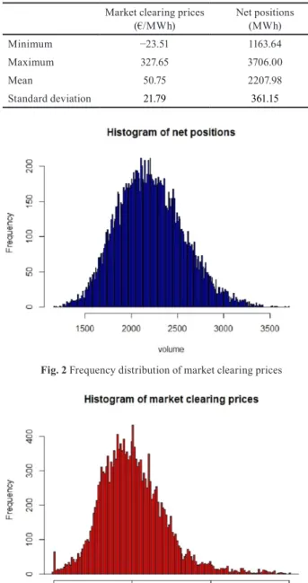
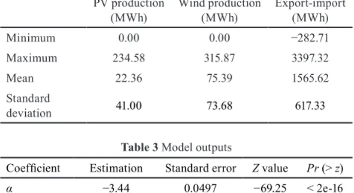
Descriptive statistics for period DAM prices and net positions are presented in Table 1, and their frequency his- tograms are presented in Figs. 2 and 3.

Price statistics show that there were hours during the period in which a negative price developed, and the high- est price was more than six times the average price. Based

Table 1 Descriptive statistics on prices and net positions Market clearing prices

(€/MWh) Net positions

(MWh)

Minimum −23.51 1163.64

Maximum 327.65 3706.00

Mean 50.75 2207.98

Standard deviation 21.79 361.15

Fig. 2 Frequency distribution of market clearing prices

Fig. 3 Frequency distribution of net positions Fig. 1 Sales and purchase curves and market clearing on 5/28/2018 5 p.m.

(5)

on the positions, it can be seen that they lag behind the total Hungarian demand (the average system load in the period was 5171 MWh (MAVIR Zrt., 2020)), since traders also have other organized (futures, intraday) and over-the- counter (or bilateral) purchasing opportunities.

Descriptive statistics of control variables (hourly photovoltaic and wind production, export-import) are shown in Table 2. In the period under review, the maximum available cross-border and wind capacities were stable, while the installed solar capacities increased significantly by 2018. In the case of photovoltaic production, the mean and standard deviation values can be interpreted to a lim- ited extent due to the lack of overnight production.

The reason for the logarithmic interpretation applied to bid-ask-spread in the model is that it has a very heavy right-tail and is always positive, so taking its logarithm significantly improves the performance of the model.

4 Results

This section summarises the results of the empirical study:

the values taken by the coefficients of the variables, the results of the multicollinearity test between the explanatory variables, and the predictive power of the model.

The estimation results of the model are summarised in Table 3. Significance results can be interpreted in the usual way: estimated parameters are asymptotically normally distributed, and our sample is large enough to assume that the Z score shows significance.

It can be seen that liquidity, export-import and PV production variables significantly influence the appearance of price spikes. Interestingly, the coefficient of PV and wind power production is negative, which is due to the

fact that sunny and windy hours, when power plants pro- duce around maximum capacity, are easier to predict than during periods of lower production with variable sun and wind conditions (da Silva et al., 2015). In Hungary, PV exceeds the installed capacity of wind turbines; therefore, its impact on price spikes is also greater. More significant exports increase the likelihood of price spikes, indicating that bottlenecks in foreign markets cause some of the price spikes. Finally, the effect of the bid-ask spread is positive, which means that in periods when price spikes develop, the sale and purchase curves are steeper (more inelastic) around the optimum.

The Variance Inflation Factor (VIF) indicator was used to test multicollinearity. The VIF is a score of how much the variance of a regression coefficient is inflated due to multicollinearity in the model. The method tests the correlation of each explanatory variable, by linear regression models, including all the explanatory variables of the original model. Afterwards, the VIF factor is calculated by Eq. (8):

VIF_i Ri

= + 1

1 ² (8)

where R_i² is the coefficient of determination of the linear regression model.

The VIF for the bid-ask spread was 1.02, for PV production: 1.07, for wind production: 1.03, and for export-import: 1.09. The VIF scores for all the control variables of the model are less than 5, which is a commonly used cut-off. This value indicates that the hypothesis of multicollinearity between the model's predictors is rejected.

We also report the correlation matrix of the explanatory variables in Table 4 in the Appendix. The strongest correlation (0.27) is between photovoltaic production and the difference of export and imports.

We also address endogeneity by including the correlation of the residuals and the explanatory variables in the matrix. The correlations are low enough to assume that no endogeneity issues arise in the model.

It is important to note that the variables used in the model may not be independent of each other in other coun- tries' markets. The small impact of renewables on sale curves may be due to the feed-in tariff support system.

Thus, renewable producers do not appear as strategic players in the market.

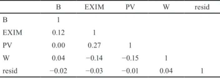
The most commonly used approach to measuring the predictive power of a logit model is to measure the area under the Receiver Operating Characteristic (ROC) curve.

It plots two parameters as results of a model: the false

Table 2 Descriptive statistics on control variables PV production

(MWh) Wind production

(MWh) Export-import (MWh)

Minimum 0.00 0.00 −282.71

Maximum 234.58 315.87 3397.32

Mean 22.36 75.39 1565.62

Standard

deviation 41.00 73.68 617.33

Table 3 Model outputs

Coefficient Estimation Standard error Z value Pr (> z)

α −3.44 0.0497 −69.25 < 2e-16

β_B*** 0.69 0.0368 18.68 < 2e-16

β_EXIM*** 0.56 0.0403 13.80 < 2e-16

β_PV*** −0.49 0.0599 −8.20 2.44e-16

β_W −0.04 0.0392 −1.14 0.253

(***) The variable is significant below the 1% significance level.

(6)

positive rate, versus the true positive rate at different classification thresholds. The ROC curve based on the results of the model is shown in Fig. 4.

Indicators often used to interpret predictive performance are the area under the ROC curve: AUC-ROC (Area Under the ROC Curve) and the Gini coefficient calculated from it. The value of the AUC_ROC indicator can be between 0.5 and 1, where 0.5 is the random classification, and 1 is the functional relationship. The Gini Coefficient has a possible range of [−1,1], and it serves a purpose to nor- malize the AUC in a way that random classifier scores 0, while a perfect classifier scores 1. The model reported in the article has an AUC-ROC value of 0.75 and a Gini coefficient of 0.5, and it would have classified the given value into average and price spike categories well in 96 percent of the periods in the total sample.

The main scientific contribution of the paper is to measure the effect of market liquidity, so the question arises as to what extent the predictive power is due to the main explanatory variable bid-ask spread and to what extent the control variables. Therefore, a model was also run in which the only explanatory variable was the bid-ask spread, and the control variables were omitted. The model yielded an AUC-ROC of 0.69 and a Gini of 0.38, which means that the contribution of market liquidity to good prediction performance is significant.

In order to complete a robustness check, we have modified the regression specification and built a model using another liquidity measure that we have developed, as the primary dependent variable. The churn ratio is a commonly used measure of liquidity in the commod- ity markets and in particular in the electricity markets as well (Agency for the Cooperation of Energy Regulators/

Council of European Energy Regulators, 2015). The churn ratio is calculated for both the demand and supply curves separately resulting two new liquidity indexes. The model reported in the article including the demand side churn rate as the primary dependent variable has a Gini coefficient of 0.35. The model using the supply side churn rate has a Gini coefficient of 0.39. Although, all the variables of the model remained positive and significant the model proved to be less efficient as the main model presented in this article. Nevertheless, the coefficients proved to be plausible and robust, which implies structural validity.

5 Conclusion

This article examined, within a logit framework, the extent to which market liquidity, renewable production, and the net export-import contributed to daily price spikes in the HUPX DAM market in 2017 and 2018. Based on the results, two main lessons can be identified. On the one hand, the explanatory variables are not correlated, i.e. the fundamental variables (renewable production, cross-border flows) are not responsible for the change in the slope of the sales and purchase curves around the optimum. On the other hand, these variables can be used to build a model with high predictive power, in which, also, the applied market liquidity is one of the strongest predictors.

One of the biggest challenges in electricity market price forecasting is dealing with extreme values. The results of the article suggest that in addition to the fundamental variables traditionally used, it would be worthwhile to display the characteristics of sale and purchase curves in the models in the future, as it may have a significant added value in predicting price spikes. The article used the most straightforward possible indicator to display the curves and thus achieved a model with high explanatory power. Although the results of the article are theoretical, they can offer strong practical motivation for traders to supplement their current forecasting models with information from the bid curve. The most important future research direction is the development of indicators that can capture the characteristics of the curves in a more sophisticated way and their incorporation into forecasting.

Acknowledgement

This work was supported by the ÚNKP-19-3 New National Excellence Program of the Ministry for Innovation and Technology.

False positive rate

True positive rate

0.0 0.2 0.4 0.6 0.8 1.0

0.00.20.40.60.81.0

Fig. 4 ROC curve

(7)

References

Agency for the Cooperation of Energy Regulators/Council of European Energy Regulators (ACER/CEER) (2015) "Annual Report on the Results of Monitoring the Internal Electricity and Natural Gas Markets in 2014", ACER/CEER, Ljubljana, Slovenia / Brussels, Belgium.

https://doi.org/10.2851/525797

Alem, Y., Beyene, A. D., Köhlin, G., Mekonnen, A. (2016) "Modeling household cooking fuel choice: A panel multinomial logit approach", Energy Economics, 59, pp. 129–137.

https://doi.org/10.1016/j.eneco.2016.06.025

Bevin-McCrimmon, F. Diaz-Rainey, I., McCarten, M., Sise, G.

(2018) "Liquidity and risk premia in electricity futures", Energy Economics, 75, pp. 503–517.

Bierbrauer, M., Menn, C., Rachev, S. T., Trück, S. (2007) "Spot and derivative pricing in the EEX power market", Journal of Banking

& Finance, 31(11), pp. 3462–3485.

https://doi.org/10.1016/j.jbankfin.2007.04.011

Biskas, P. N., Chatzigiannis, D. I., Bakirtzis, A. G. (2013) "Market cou- pling feasibility between a power pool and a power exchange", Electric Power Systems Research, 104, pp. 116–128.

https://doi.org/10.1016/j.epsr.2013.06.015

Boogert, A., Dupont, D. (2008) "When Supply Meets Demand: The Case of Hourly Spot Electricity Prices", IEEE Transactions on Power Systems, 23(2), pp. 389–398.

https://doi.org/10.1109/tpwrs.2008.920731

Christensen, T. M., Hurn, A. S., Lindsay, K. A. (2012) "Forecasting spikes in electricity prices", International Journal of Forecasting, 28(2), pp. 400–411.

https://doi.org/10.1016/j.ijforecast.2011.02.019

Diallo, A., Kácsor, E., Vancsa, M. (2018) "Forecasting the Spread Between HUPX and EEX DAM Prices the Case of Hungarian and German Wholesale Electricity Prices", In: 15^th International Conference on the European Energy Market (EEM), Lodz, Poland, pp. 1–5.

https://doi.org/10.1109/EEM.2018.8469921

da Silva, N. P., Rosa, L., Zheng, W., Pestana, R. (2015) "Wind Power Forecast Uncertainty Using Dynamic Combination of Predictions", Periodica Polytechnica Electrical Engineering and Computer Science, 59(3), pp. 78–83.

https://doi.org/10.3311/PPee.8575

de Menezes, L. M., Russo, M., Urga, G. (2019) "Measuring and Assessing the Evolution of Liquidity in Forward Natural Gas Markets:

The Case of the UK National Balancing Point", The Energy Journal, 40(1), pp. 143–170.

https://doi.org/10.5547/01956574.40.1.lmen

Fox, J., Andersen, R. (2006) “Effect Displays for Multinomial and Proportional-Odds Logit Models”, Sociological Methodology, 36(1), pp. 225-255.

https://doi.org/10.1111/j.1467-9531.2006.00180.x

Frestad, D. (2012) "Liquidity and dirty hedging in the Nordic electricity market", Energy Economics, 34(5), pp. 1341–1355.

Füzi, Á., Mádi-Nagy, G. (2014) "Flow-based Capacity Allocation in the CEE Electricity Market: Sensitivity Analysis, Multiple Optima, Total Revenue", Periodica Polytechnica Social and Management Sciences, 22(2), pp. 75–85.

https://doi.org/10.3311/PPso.7259

Halkos, G. (2019) "Examining the level of competition in the energy sector", Energy Policy, 134, Article number: 110951.

https://doi.org/10.1016/j.enpol.2019.110951

Huisman, R., Mahieu, R. (2003) "Regime jumps in electricity prices", Energy Economics 25(5), pp. 425–434.

https://doi.org/10.1016/S0140-9883(03)00041-0

Hungarian Power Exchange (HUPX) "Energy Businass Motion: DAM - Aggregated data", [online] Available at: https://hupx.hu/en/market- data/dam/aggregated-data [Accessed: 18 June 2020]

Hurn, A. S., Silvennoinen, A., Teräsvirta, T. (2016) "A Smooth Transition Logit Model of the Effects of Deregulation in the Electricity Market", Journal of Applied Econometrics, 31(4), pp. 707–733.

https://doi.org/10.1002/jae.2452

Ibikunle, G., Gregoriou, A., Hoepner, A. G. F., Rhodes, M. (2016)

"Liquidity and market efficiency in the world’s largest carbon market", The British Accounting Review, 48(4), pp. 431–447.

https://doi.org/10.1016/j.bar.2015.11.001

Janczura, J., Trück, S., Weron, R., Wolff, R. C. (2013) "Identifying spikes and seasonal components in electricity spot price data: A guide to robust modeling", Energy Economics, 38, pp. 96–110.

Kyle, A. S. (1985) "Continuous Auctions and Insider Trading", Econometrica, 53(6), pp. 1315–1335.

https://doi.org/10.2307/1913210

Kyritsis, E., Andersson, J., Serletis, A. (2017) "Electricity prices, large- scale renewable integration, and policy implications", Energy Policy, 101, pp. 550–560.

https://doi.org/10.1016/j.enpol.2016.11.014

Manner., H., Türk, D., Eichler, M. (2016) "Modeling and forecasting multivariate electricity price spikes", Energy Economics, 60, pp. 255–265.

Marossy, Z. (2012) "Az Extrém Ármozgások Statisztikai Jellemzői a Magyar Áramtőzsdén" (The statistical characteristics of extreme price movements in the Hungarian power exchange), Vezetéstudomány, 43(5), pp. 14–24. (in Hungarian)

https://doi.org/10.14267/veztud.2012.05.02

MAVIR Zrt. "Hungarian Power System actual data", [online] Available at: https://www.mavir.hu/web/mavir-en/hungarian-power-system- actual-data [Accessed: 08 July 2020]

Mileta, D., Šimić, Z., Skok, M. (2011) "Forecasting prices of electricity on HUPX", In: 8^th International Conference on the European Energy Market (EEM), Zagreb, Croatia, pp. 204–208.

https://doi.org/10.1109/EEM.2011.5953009

Sousa, J., Mendes, V. M. F. (2004) "The Iberian Electricity Market-Impacts on power producer profits. consumer surplus and social welfare in the wholesale market", presented at ENERGEX - 10^th International Energy Forum – Energy & Society, Lisbon, Portugal, May, 3-6, 2004.

(8)

Szőke, T., Hortay, O., Balogh, E. (2019) "Asymmetric price transmission in the Hungarian retail electricity market", Energy Policy, 133, Article number: 110879.

https://doi.org/10.1016/j.enpol.2019.110879

Trueck, S., Weron, R., Wolf, R. (2007) "Outlier Treatment and Robust Approaches for Modeling Electricity Spot Prices", In: 56^th Session of the Internatioanal Statistical Institute, Invited Paper Meeting IPM71, Lisbon, Portugal, MPRA Paper number: 4711.

[online] Available at: https://mpra.ub.uni-muenchen.de/4711/

[Accessed: 18 June 2020]

Weron, R. (2008) "Market price of risk implied by Asian-style electricity options and futures", Energy Economics, 30(3), pp. 1098–1115.

Ziel, F., Steinert, R. (2016) "Electricity price forecasting using sale and purchase curves: The X-Model", Energy Economics, 59, pp. 435–454.

Appendix

Table 4 Correlation of the explanatory variables and the residual

B EXIM PV W resid

B 1

EXIM 0.12 1

PV 0.00 0.27 1

W 0.04 −0.14 −0.15 1

resid −0.02 −0.03 −0.01 0.04 1