IMPACT ASSESSMENT OF INCREASING THE 20%
GREENHOUSE GAS REDUCTION TARGET OF THE EU FOR HUNGARY
EXECUTIVE SUMMARY
Study was commissioned by the Hungarian Ministry of National Development and financed by the European Climate Foundation
Regional Centre for Energy Policy Reasearch
2
INTRODUCTION
This study has the objective to analyse the impacts on the Hungarian economy of a higher EU GHG (greenhouse gas) reduction undertaking for 2020, namely increasing the GHG reduction target to 20% and to 30% relative to 1990. In order to achieve this objective, we quantify the costs/benefits of these increased undertakings for the various sectors of the Hungarian economy.
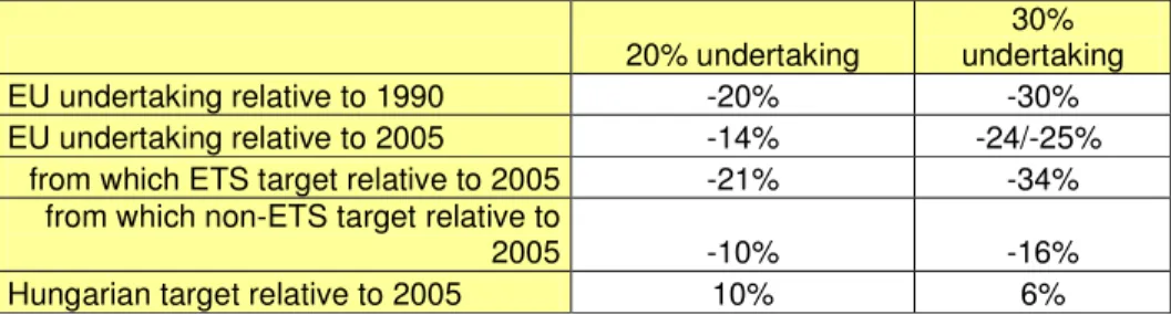
Table i: Distribution of undertakings by sectors in the cases of 20% and 30% EU targets
20% undertaking
30%
undertaking
EU undertaking relative to 1990 -20% -30%
EU undertaking relative to 2005 -14% -24/-25%
from which ETS target relative to 2005 -21% -34%
from which non-ETS target relative to
2005 -10% -16%
Hungarian target relative to 2005 10% 6%
Source: DG Climate
It is important to know that the EU regulation divides national economy sectors into two groups from the viewpoint of GHG abatement target. On the one hand, the EU undertook a target for ETS1 companies. Within this undertaking, the emission reductions of companies are independent from national decisions. These companies may purchase emission quotas adequate to their emissions partially on auctions, and partially free of charge, thus the decision on the CO2 amount they abate and the quota amount they buy is made by them. This also means that both expenses and quota revenues occur at the companies. In the other sectors of the economy (non-ETS sectors), countries have national targets, for the fulfilment of which national governments are responsible. The carbon market of this segment is called ESD2 market, where only governments may trade, i.e. revenues are gained by and expenses are charged to governments.
The first part of the study assesses the impact of the 30% target on the sectors falling under the European Emission Trading Scheme (EU-ETS). The electricity sector is examined with a regional electricity market model developed by REKK. In the case of energy intensive ETS sectors, we analysed these sectors’ exposure to the carbon leakage effect, i.e. the risk of transferring emissions to other non-taxed regions, in other words, how much they lose from their competitiveness relative to non-EU countries and what impacts it may have on the given sector.
1 ETS: emission trading scheme. ETS includes energy transformation sectors (electricity, refining), energy intensive sectors (steel, cement, ceramics and glass production, paper industry) however, since 2013 also includes given sectors of chemical industry and aviation. All the other sectors are called non-ETS sectors.
2 ESD: Emission Sharing Decision
3 Top GHG emitters of non-EU-ETS sectors are the building stock of the household, the public and the tertiary sectors, transport and agriculture, and significant GHG is emitted from municipal solid waste and sewage treatment. On the one hand, we model the future business- as-usual evolution of these sectors (BAU scenarios) while on the other hand, we examine two reduction scenarios, where the GHG emission is lower than one. For the given sectors, we define GHG abatement potentials and the marginal costs thereof, which may provide valuable information on the GHG abatement potentials of these sectors. Accordingly, we have carried out an in-depth modelling for the sectors listed above, while prepared only a BAU scenario based on a historical trend for the remaining sectors characterised by lower emission in order to be able to compile a complete GHG balance for the period from 2013 to 2020.
Consequently, our goal was to prepare a decision-preparing document that tries to quantify the expected costs and benefits of a higher EU-level GHG reduction target for Hungary. With regard to benefits, we give estimates on direct benefits. These are quota revenues, direct employment impacts in household and tertiary sectors as well as reduction in natural gas consumption3 in the various scenarios. Accordingly, the analysis is not comprehensive from this aspect since indirect impacts are not quantified.
In the following we sum up the key results. First, we give a sectoral introduction on the applied methodology and the main assumptions, which is followed by our GHG estimates for the various sectors and scenarios. We also give an aggregate assessment of the non-ETS sector, since these sectors constitute a separate carbon market in line with the logic of the European regulation. The summary is completed by the evaluation of the aggregate economic impacts. Above all, however, we give a short overview of the features and key figures of the domestic GHG emissions.
3 Social benefits here may occur as the mitigation of Hungary’s one-sided gas import dependency.
4
EVOLVEMENT AND COMPOSITION OF DOMESTIC GHG EMISSION
In order to forecast future GHG emissions, it is important to be aware of the historical emissions of the various gases and sectors.
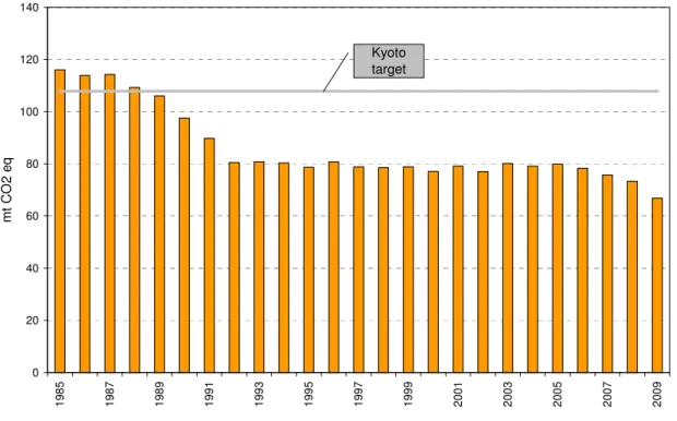
In 2009, Hungary emitted 66.837 million tonnes CO2 equivalent green house gas excluding absorbers. Including absorbers, this value amounts to 63.792 million tonnes, which is 43.3%
lower than the average of the years 1985-87, which was the base for Hungary’s 6%
undertaking in the Kyoto Protocol. Following the economic collapse, emission stagnated between 1999 and 2005, which was followed by a decline since 2005. Considering the whole period, the most significant reduction occurred in CO2 emission.
Figure i: Hungary’s GHG reduction between 1985 and 2009 (excluding LULUCF4)
0 20 40 60 80 100 120 140
1985 1987 1989 1991 1993 1995 1997 1999 2001 2003 2005 2007 2009
mt CO2 eq
Kyoto target
Source: Hungarian GHG Inventory
The most significant greenhouse gas is carbon-dioxide that accounts for 75% of the 2009 emission. CO2 primarily derives from the combustion of fossil energy carriers. CO2 is followed by methane (13%), and nitrous oxide (11%). The primary sources of methane emission are waste deposits and animal farming, however, fugitive gas emissions from fuels are considerable as well. Nitrous oxide emission primarily derives from chemical fertilizer use
4 Land use, land use change and forestry
5 and nitric acid production as well as from road transport. Although the share of F-gases (HFCs, PFCs and SF6) is not significant in the total emission, the amount used is continuously rising and their share dynamically grows due to their high global warming potential (GWP).
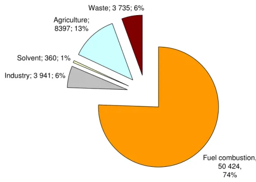
Within the emitting sectors, energy production is responsible for more than three quarters of emissions, which is followed by agriculture with 13%. Industry and waste have nearly the same contribution (6% each) to the total emission.
Figure ii: Hungary’s GHG emission according to sectors in 2009 (excluding LULUCF), thousand tonnes CO2eq, and %
Waste; 3 735; 6%
Agriculture;
8397; 13%
Solvent; 360; 1%
Industry; 3 941; 6%
Fuel combustion, 50 424,
74%
Source: Hungarian GHG Inventory
ETS installations were responsible for average 35-36% of the total domestic GHG emission between 2005 and 2009. Since there will be a small increase in the number of installations falling under ETS in 2013, this share is expected to grow to a small extent.
6
ELECTRICITY SECTOR
The study gives a detailed analysis on the effect of a lower EU ETS cap on the Hungarian electricity sector.
The study introduces five unique scenarios, which differ in total quota amount, the share of renewable capacities and the intensity of energy efficiency measures. The following table shows the denominations of the scenarios and the main assumptions.
Table ii: Main scenario assumptions to 2020 Assumptions Scenario
Quota Share of renewables Electricity consumption
BAU
Quota equals the second ETS period emissions
Half of the renewable investments set in member state NREAP-s are realized
No significant energy efficiency measures are introduced in the
analysed countries
REF20
Quota reduction (-21% compared
to 2005 emissions)
Renewable energy generated as set in the Renewable
Energy Directive
No significant energy efficiency measures are introduced in the
analysed countries
REF20+
Quota reduction (-21% compared
to 2005 emissions)
The full renewable investments set in member state NREAP-s
realized
Profitable energy efficiency programmes are realised in the
analyzed countries
CC30
Quota reduction (-34% compared
to 2005 emissions)
Renewable energy generated as set in the Renewable
Energy Directive
No significant energy efficiency measures are introduced in the
analysed countries
CC30+
Quota reduction (-34% compared
to 2005 emissions)
The full renewable investments set in member state NREAP-s
realized
Profitable energy efficiency programmes are realised in the
analyzed countries
*NREAP: National Renewable Energy Action Plan Source: REKK assumption
The following table shows the parameter assumptions (EUA price, electricity consumption and spread of renewable sources) to the given scenarios we defined.
Table iii: Assumptions for the various scenarios for 2020 Assumptions for 2020 Scenario EUA price, €/t (2008
base)
Renewable-based electricity production in Hungary, TWh
Gross electricity consumption,GWh
BAU 13.0 4 220 48 466
REF20 16.5 4 809 48 466
REF20+ 10.5 5 597 45 751
CC30 36.0 4 809 48 466
CC30+ 30.0 5 597 45 751
Source: REKK
7 One of the most important of these parameters is the quota price. We assume that there is no quota reduction in the BAU scenario, which results in the carbon dioxide quota price’s remaining at 13 €/t5. However, the cap becomes lower by 21% relative to 2005 in the REF20 scenario, and also the period after 2020 will witness lower cap which may result in higher quota prices. Accordingly, the quota price by 2020 will grow to 16.5 €/t6 at 2008 prices based on the PRIMES7 model. In the CC30 and CC30+ scenarios, the cap is still lower, which results in a higher quota price, namely the price would be 36.0 €/t8 (CC30), and 30.0 €/t9 (CC30+), respectively by 2020. Since the electricity consumption will be lower on the one hand, and the share of renewables will grow on the other hand in the REF20+ scenario therefore the quota price is expected to be lower. We assume that the quota price will be 10.5
€/t at 2008 prices.
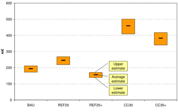
We can forecast the quota revenues and estimate the production costs of electricity for Hungary in the case of the above defined scenarios. The figure below shows the average, lower and upper estimates of annual auction revenues in Hungary.
Figure iii: Average, lower and upper estimates of the auction revenues, m€
0 100 200 300 400 500 600
BAU REF20 REF20+ CC30 CC30+
m€
Average estimate
Upper estimate
Lower estimate
Source: REKK calculation
5 Source: COM 265/2010, Staff working document, Part II.
6 It is adequate to the WAM or REF scenarios in the documents of the EU Commission.
7 Source: Templates for data related to policies and measures, and projected GHG emissions, to be reported under Article 3(2) of the Monitoring Mechanism Decision (Commission Decision 280/2004/EC)
8 This price equals the EU Roadmap reference scenario, which calculates with a 34% reduction by 2030, so the 2030 prices can be applied to 2020.
9 It is adequate to the COM -30% scenario, during which sigificant energy efficiency projects are realised.
8 We estimate the effect of the various scenarios on the electricity market with the help of a regional power market model, which simultaneously simulates the electricity markets and the commercial flows of Central and South European countries. The following table sums up the three most important factors that serve as a basis for evaluating the scenarios. These are natural gas consumption of electricity production, average auction revenue and electricity price increased by renewable subsidies.
Table iv: Summary of scenarios
BAU REF20 REF20+ CC30 CC30+
Natural gas consumption,
mcm 4756 4712 3084 6717 5368
Average auction revenue,
m€ 194 246 157 459 383
Electricity price, €/MWh 76.1 77.3 70.0 86.8 81.0 Source: REKK calculation
Based on the two comparable scenario pairs (REF20 vs. CC30; and REF20+ vs. CC30+), the following statements can be made.
• A higher EU-level emission reduction target would increase the natural gas consumption of the electricity sector by 40-70%, which is very significant. This primarily comes from the fact that higher CO2 prices provide a competitive edge to the domestic gas-fired power plants relative to the coal-fired ones.
• The following figure displays the additional government revenues from quota sales and the increase in the expenses to be paid by electricity consumers, i.e. by how much electricity customers would pay more for purchasing electricity due to a narrow ETS cap. As the figure shows a narrow ETS cap would result in an additional auction revenue amounting to around 200 million EUR in both cases. However, the electricity expenses of consumers would grow by 4-500 m€, which is more than double the aditional auction revenues. Accordingly, while a narrow ETS cap could be favourable exclusively from budgetary point of view, its total welfare effect is dubious, and depends largely on the efficiency of the use of the aforementioned excess revenue.
9 Figure iv: Comparison of auction revenues and total electricity procurement expenses for narrow ETS
cap, m€, 2008 prices
0 50 100 150 200 250 300
450 455 460 465 470 475 480 485 490 495 500
Difference of total electricity procurement expenses, m€
Difference of total revenues of quata sales, m€
CC30+
vs.
REF20+
CC30 vs.
REF20
Source: REKK calculation
10
NON-ENERGY INDUSTRIAL ETS SECTORS
The methodology of analysis accepted by the Commission extends the effects of the EU climate policy to the demand and supply sides of non-energy industries under ETS. On the one hand, (on demand side) it cumulates the direct and indirect industrial CO2 costs incurring in the ETS sector and on the other hand (on supply side) examines to what extend the given sectors can transfer these costs to their customers. The transfer depends on the price increase, is limited by the competition in supply and the demand response depending on the price sensitivity of consumers. Therefore, non-EU non-ETS companies are significant competitors to the industries of the EU ETS sector on the supply side.
Literature evidence shows that the current regulatory environment, which manifests in relatively low CO2 prices and no border adjustment of non-EU import prices, has only limited effects on European industries under ETS. Cement, iron and steel industries face the highest relative risks of losing market share: cement is the most CO2-intensive of all non-energy industries under ETS, and iron and steel industries are the most exposed to foreign trade of goods produced free of CO2 costs outside of the EU.
We find risks for the Hungarian industries lower than the overall EU pattern. CO2 intensity of coke and oil refinery production, curiously, looks much smaller in Hungary than in the European industry. This is an issue that is to be verified by data owners. Moreover, European industries under ETS overall are more than twice as threatened by foreign trade than the Hungarian ones, according to our results. Exposure to foreign trade is especially low in the Hungarian coke, ceramics, oil refinery, iron and steel industries compared to their European peers. The following graph summarizes our results for the potential risks of carbon leakage from the Hungarian ETS industries under the “20%” or “30%” European climate policy.
11 Figure v: Risk of carbon leakage within Hungarian ETS industries on the basis of their foreign trade intensity and the maximum cost of their own emissions, 2008, 100% auctioning of EUA at prices 25€/t and
38.5 €/t
0%
5%
10%
15%
20%
25%
30%
35%
40%
45%
50%
55%
60%
65%
70%
0% 5% 10% 15% 20% 25% 30% 35% 40%
foreign trade intensity maximum cost of own emissions as percent of total value added
5%
30%
10% 30%
coke
cement.lime
Brick, ceramics
Refinary iron, steel
paper, pulp Glass 16,5€/t
36 €/t
indicative treshold values for risk of carbon leakage
stand alone treshold values for risk of
carbon leakage
Source: REKK calculation from CITL and EUROSTAT data
We draw attention to the fact that low trade intensity gives way to industries to apply profit maximizing prices, which means that they are able to raise their prices by all the CO2 costs irrespective of the CO2 quota allocation regime. So, compared to their European peers, Hungarian industries are better positioned to raise their prices with the opportunity cost of their CO2 quotas, regardless of the freely allocated amount of CO2 emission quotas.
12
ENERGY EFFICIENCY OF BUILDINGS
There are huge energy saving potentials in the building stocks of both residential and services sectors of Hungary, which also imply a significant GHG emission reduction opportunity. The above statement was confirmed by numerous studies, such as NEGAJOULE (2011), Envincent (2011), HUNMIT (2009), and it is also reflected by the figures of the database of the Directorate General Energy of the European Commission on energy saving potentials10. We have used the HUNMIT model, provided by the Ministry of National Development, for the estimation of future GHG emissions11 of (both residential and public) buildings in this study. The building energy efficiency option of the HUNMIT model has been used, however, we have updated several input parameters (energy prices, current emission levels, schedule of measures) and we have modified the applied method as well. Within the latter, the scarcity of financial resources has been taken into account, as well as realistically realisable building retrofitting programs based on profitability indices calculated upon net present value for the whole lifespan of investments. The above changes are needed because the biggest obstacle to reduction is the lack of resources, although it is obvious that there are significant GHG emission abatement potentials in the residential and tertiary sectors. Based on historical data of energy efficiency investments on buildings, upon the previously mentioned surveys, in line with our calculations it is clear that the level of building retrofitting investments over the next decade is likely to be suboptimal without governmental involvement. As a result, the limits of the energy efficiency investment programs for buildings will rather be determined by the available resources; therefore, we have examined the following two scenarios:
• Reference (REF) scenario: in line with the REF20+ scenario, the available funding for building retrofitting programmes is covered by the ETS quota revenues. The estimated average revenue of this scenario is 157 million € (in line with the REF20+ scenario), which accounts for 43 billion HUFs. We assume that the subsidy intensity is 40%, i.e.
40 of the 100 units of investment cost are paid as a state subsidy. This also implies that the total amount of 43 billion HUFs could induce investments of as much as 105 billion HUFs. This investment size includes the additional investments, namely the projects in addition to the BAU projects (autonomous investments).
10 http://www.eepotential.eu/esd.php
11 The HUNMIT, prepared in 2009 for the Ministry of Environemental Protection and Rural Development (KvVM) by a consortium led by the consulting company Ecofys, is a model prepared for Hungary with the aim of estimating greenhouse gas emissions, abatement potentials till 2025 in the following sectors: households, services, industry, transport, energy and waste.
13
• In the Reference + (REF+) scenario, we applied the same assumption except for using here the REF30+ electricity scenario as a base implying a revenue of 383 million € (103 billion HUFs), which shifts the achievable investment level to 258 billion HUF.
We furthermore assume that the resources available are allocated between the two subsectors (household buildings and the building stock of the tertiary sector) in a cost effective way, i.e.
we do not label subsidies between the two subsectors but choose cost effective solutions in line with the limited resources. For these cases, we set the discount rate to 6% (equal to the social discount rate), since we assumed that the above mentioned resources are available at state budget level.
However, there are considerable uncertainties inherent in our scenarios: on the one hand, the uncertainty of the ETS quota price, on the other hand, the governmental decision whether the ETS quota revenues are really used for funding such programmes.
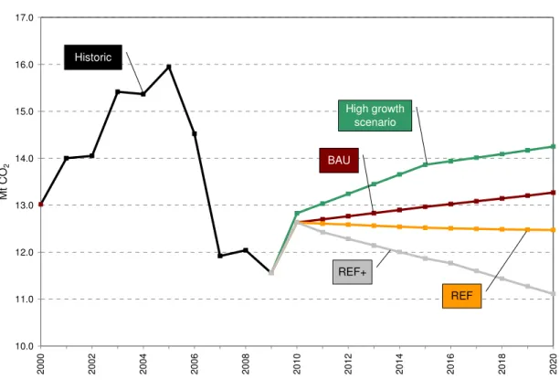
The following figure illustrates the emission estimates for the baseline (BAU), REF and REF+ scenarios. The figure includes direct emissions only (excluding emissions linked to electricity and district heat consumption).
Figure vi: CO2 emission in household and services building sectors (Mt CO2)
10.0 11.0 12.0 13.0 14.0 15.0 16.0 17.0
2000 2002 2004 2006 2008 2010 2012 2014 2016 2018 2020
Mt CO2
Historic
BAU
High growth scenario
REF+
REF
Source: Enerdata and REKK calculations
The figure above shows that the estimated emission paths of the two subsectors of the BAU scenario produce a slightly increasing trend, which is offset by the significant CO2 emission
14 reduction estimates of the REF and REF+ scenarios. In the case of a fast economic growth (in which the services sector reaches the pre-crisis activity level in 2015), greenhouse gas emission levels are lagging far behind the 2005 levels – the base year of emission abatements.
Relative to the base year of 2005, emissions are lower by 17% in the BAU scenario, by 22%
in the REF scenario and by 30% in the REF+ scenario. Even the quick-paced scenario, which produces a 10% reduction, lags behind the 6% growth limit of the 30% EU target. The main reason behind the differences is the considerable reduction in emissions between 2005 and 2009, owing to several factors. Differences are partly explained by the effect of the crisis, and partly by the higher values of the annual mean temperature.
The benefits of building renovations were quantified following three dimensions:
• firstly, the revenue from carbon quota sold on directly available ESD12 market,
• secondly, the employment impacts of the programmes, and
• thirdly, natural gas savings due to the programmes.
When giving estimates of carbon quota revenue, we have applied the PRIMES model’s quota prices. The PRIMES model projected 4 and 30 euro/tCO2 prices for the ESD markets for the 20% and 30% EU targets, while in the case of a closed EU ESD market the carbon prices reaches 55 euro. We have applied the specific employment values of the (2010) Ürge-Vorsatz study, which has calculated the investment costs of bigger building retrofitting programmes for Hungary and their impact on employment. Natural gas savings are direct results of the modelled building refurbishment programmes.
Table v: Quantifiable costs and benefits of building refurbishment programmes in 2020 Direct
employment impact (thousand people/year)
Total (direct and indirect) employment impact (thousand
people/year)
Natural gas savings
(mcm)
Average investment
level, M€
State subsidy
M€
ESD quota revenue,
m€
20% target 10-13 15-19 335 393 157 53
30% target 25-33 36-42 1053 958 383 394
Difference of the 20 vs 30
% targets
15-20 21-23 718 565 226 341
Source: REKK calculations
The table shows the amount of investments and the associated savings on natural gas, the ESD quota revenues and employment impacts for 2020. It can be concluded that tightening GHG emission targets resulted in a positive outcome overall in the case of all categories of building stocks. However, it is important to note that the benefits ocurring are not directly
12 Effort Sharing Decision (406/2009 EC decison of the European Parliament and of the Council)
15 linked to the investments of 2020, but these are resulted from all the (cumulative) impacts of a decade long investment programme.
16
TRANSPORT SECTOR
Based on the GHG inventory, transport sector made up 19% of the total GHG emission of Hungary and one fourth of energy emissions in 2009. This figure excludes the emission of aviation, which is not integrated but appears separately in the national inventory. Compared to other non-ETS sectors, this one is characterised not only by a significant share in the total emission but also by a dynamically growing emission and by far the highest growth rate.
Throughout a decade before the crisis (from 1998 to 2008) the total annual emission of the sector grew by as much as 5%, which exceeds the emission increase of all the other sectors.
The economic crisis had effect also on the transport sector resulting in fallbacks primarily in the emissions of road transport and aviation.
In order to model the 2020 forecast of the BAU scenario, we use an econometrically estimated passenger car forecast, which is supplemented by the statistical estimate of the freight transport volume. In determining the penetration level of the domestic passenger car stock, the applied model uses the hypothesis of convergence to the European development level, within which the effect of crisis (scarcity of financial resources) is taken into account.
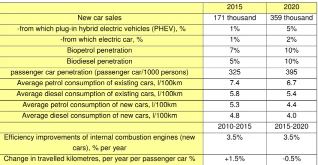
The following table contains the most important parameters of the BAU scenario.
Table vi: BAU scenario parameters for passenger transport sector
2015 2020
New car sales 171 thousand 359 thousand
-from which plug-in hybrid electric vehicles (PHEV), % 1% 5%
-from which electric car, % 1% 2%
Biopetrol penetration 7% 10%
Biodiesel penetration 5% 10%
passenger car penetration (passenger car/1000 persons) 325 395 Average petrol consumption of existing cars, l/100km 7.4 6.7 Average diesel consumption of existing cars, l/100km 5.8 5.4 Average petrol consumption of new cars, l/100km 5.3 4.4 Average diesel consumption of new cars, l/100km 4.8 4.0
2010-2015 2015-2020 Efficiency improvements of internal combustion engines (new
cars), % per year
3.5% 3.5%
Change in travelled kilometres, per year per passenger car % +1.5% -0.5%
Source: REKK assumptions
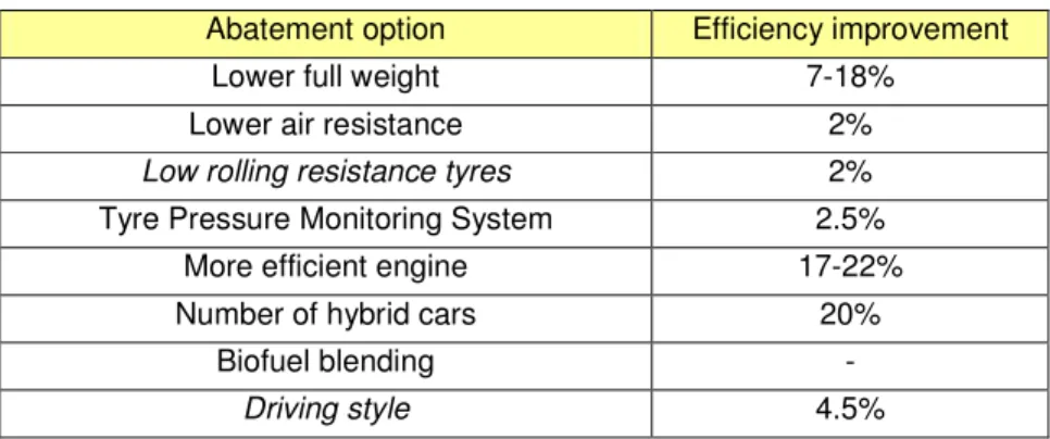
Similarly to other sectors, we examined further two scenarios (REF and REF+), which also use the abatement options of the HUNMIT model, however, the penetration level and the costs of options have been revised based on external experts’ estimates. These options along with their saving potentials are summarised in the table below.
17 Table vii: Abatement options for passenger cars
Abatement option Efficiency improvement
Lower full weight 7-18%
Lower air resistance 2%
Low rolling resistance tyres 2%
Tyre Pressure Monitoring System 2.5%
More efficient engine 17-22%
Number of hybrid cars 20%
Biofuel blending -
Driving style 4.5%
Source: REKK assumptions
We do not assume any further increase in the share of biofuel blending relative to the BAU level. We assumed in the BAU scenario that Hungary complies with the EU target for fuel blending.
Taking into account also these options, we can forecast the GHG emission paths of the three examined scenarios, which are displayed by the following figure.
Figure vii: GHG emission scenarios of transport sector.
8.8 9.1
9.6 10.0
10.5 12.2
12.7 12.8 12.9
12.7 12.8
13.2 13.5
13.8
14.2 14.3 14.4 14.4 14.4 14.4
12.6 12.8
13.0 13.2 13.3 13.3 13.2 13.1
12.8 12.6 12.2
12.6 12.9
13.2 13.4
13.7 13.7 13.7 13.6 13.5
13.3
8.0 9.0 10.0 11.0 12.0 13.0 14.0 15.0
2000 2002 2004 2006 2008 2010 2012 2014 2016 2018 2020
million ton, CO2eq
Historic
REF+
BAU
REF
Source: REKK assumptions, KSH
The figure clearly shows the increasing trend in the GHG emission of the transport sector, which was set back by the crisis for two years, even though further dynamic growth can be rendered probable since the Hungarian figures of both the number of passenger cars per thousand people and person-kilometre are still low when conmpared to the European average.
18 There is a significant GHG reduction in the reference scenario; however, a significant part of this reduction is achieved by introducingcars to the market with more efficient engines and hybrid cars, which are options with expensive abatement costs.
19
AGRICULTURE
We have given an estimate for emissions of methane and nitrous oxide originating from agriculture till 2020. It is important to note that within the agricultural sector we do not analyse emissions of land use, land use change and forestry (LULUCF) as these emissions are not included in the targeted 20% reduction of the EU.
Three scenarios have been set up for the agricultural sector. Within the BAU scenario our assumption is to calculate the effects of pre-2009 measures only, within the REF scenario impacts of post-2009 measures are taken into account, while in the REF+ scenario even post- 2010 supplementary provisions’ effects are applied. The table below gives a summary of the assumptions of three scenarios.
Table viii: Summary of changes by scenarios that are likely to take place within the agricultural sector
BAU REF REF+
Use of fertiliser 16% growth from 2009 base year to 2020
7% growth from 2009 base year to 2020
9% decline from 2009 base year to 2020 Production area of
cereals 50,000 ha growth 150,000 ha decline 200,000 ha decline Yield of industrial
plants Significant growth Moderate growth Slight increase in yield of plants Yield of vegetables Slight decline Stagnation Slight increase
Yield of pulses Stagnation Moderate growth Significant growth Area of plantation Constant decline Stagnation Slight increase Diary cattle stock Drastic decline Moderate decline Slight decline Meat cattle stock Slight growth Moderate growth Stronger growth
Sheep stock Decline Decline Stagnation after slight
drop Pig stock Drastic decline Moderate decline Moderate decline
Poultry stock No impact No impact No impact
Manure management
Moderate growth in biogas production
Moderate growth in biogas production
Significant growth in biogas production Source: REKK assumptions
Nitrous oxide emissions are likely to decline slightly till 2020 in the BAU scenario, primarily due to emission reduction of manure management, while direct and indirect soil emissions originating from grazing is predicted to change slightly as compared to 2009 levels. A significant decline can be observed in methane emissions: a drop from 123 thousand tonnes of 2009 to 107 thousand tonnes in 2020. This can be explained by a decrease in emissions from manure management as well as from animal digestion owing to the decline in number of animal stock.
20 As indirect emissions also show a slight drop, in the case of N2O, decline is even more significant in the REF scenario. This is partially offset by the increase in direct soil emissions.
As a result, emission falls from 19 thousand tonnes of 2009 to 17 thousand tonnes in 2020.
Methane emissions also indicate a downward correction as compared to the 2009 base year, however, the decline is less than in the BAU scenario. Owing to decreasing emissions of manure management and of digestion origin, methane emission drops from 123 thousand tonnes to 116 thousand tonnes in the investigated period. The reason behind the decline is the drop in number of animal stock, but to a smaller extent than it contributed to the drop in the BAU scenario.
The estimated path of the REF+ scenario indicates a similar trajectory, both in pace and magnitude, as seen in the REF scenario, although direct and indirect soil emissions decline more in the REF+ scenario than in the REF scenario. After a moderate increase in methane emissions, a slight upturn is envisaged as compared to 2009 level, however, this latter level still lags behind the average of 2005-2009. This can be explained by a slighter drop in the number of animals.
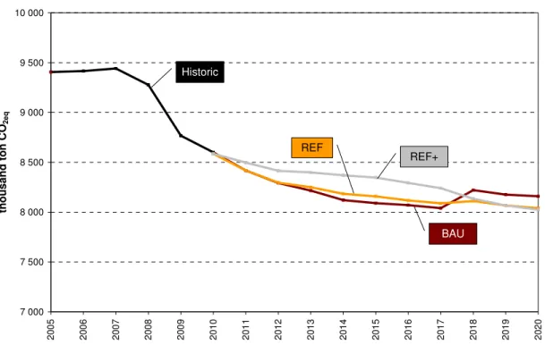
The figure below indicates the GHG emissions estimated for the three scenarios.
Figure viii: GHG emissions of the three scenarios
7 000 7 500 8 000 8 500 9 000 9 500 10 000
2005 2006 2007 2008 2009 2010 2011 2012 2013 2014 2015 2016 2017 2018 2019 2020
thousand ton CO2eq
Historic
BAU REF REF+
Sources: REKK calculation, GHG inventory
The figure above might seem surprising for the first time, since almost each year another scenario produces the lowest emission level. The reason behind is the fact that changes in emissions due to the changing number of animals and emissions fluctuating due to intensity of
21 cultivation are offsetting each other. Thus, since the decreasing number of livestock and the high fertiliser use resulting from relatively intense cultivation in the BAU scenario, as well as a slighter drop in the number of livestock and a relatively bigger drop in the use of fertilisers in the REF+ scenario compensate each other, there is no significant difference in the three scenarios’ GHG emission levels.
22
WASTE MANAGEMENT
Taking into account the current logic of GHG accounting, as for municipal solid waste (MSW) management, we have primarily included methane originating from waste deposit and carbon-dioxide of combustion origin (excluding combustion of compound substances of organic compound) in the emissions of the waste management sector.
The quantity of municipal solid waste has fluctuated to a great extent over the last two decades including a stagnating period with a drop at the end of the ’90s, which was followed by a slight upward trend since 2000. The quantity of municipal solid waste per head lags well behind EU-15 average, as well as from EU-27 average. Within Hungary, the average municipal solid waste per head was around 450 kg in 2008, while reached 550 kg in EU-15 countries at the same time. When investigating last years’ trends, it can be concluded that there is no catch-up: the difference between Hungary and old EU countries remained stabile.
The following scenarios have been defined for making forecasts on waste management:
Table ix: Waste management GHG scenarios Scenario Source of waste Ratio and technology
of waste deposit Tendencies of utilisation
BAU
Production: slight downturn in line with the trend of the last decade;
Consumption: slight upturn
Deposit: majority of proportion, combustion
capacity does not increase
Slight increase, a bit late as compared to EU regulation
REF
Deposit declines substantially, in favour
of incineration
In line with EU regulation from all aspects
REF+
Production: a higher drop as compared to previously seen;
Consumption:
stabilisation
Deposit shows a slight drop, after prevention
and utilisation
Grows mainly in line with EU regulation, sometimes it may
remain below those (e.g.
MSW) Source: REKK assumptions
Accordingly, first the expected quantity of waste is estimated, which is followed by the prognosis for changes in waste mix. Both estimations are based on the estimates of the National Waste Management Plan (NWMP). GHG emissions can be calculated upon the IPCC guidelines (2006), in which estimations for methane emission of deposit and CO2
emission of combustion origin were calculated separately.
23 Figure ix: Waste management GHG scenarios
1.5 1.7 1.9 2.1 2.3 2.5 2.7 2.9 3.1
2008 2009 2010 2011 2012 2013 2014 2015 2016 2017 2018 2019 2020 Mt CO2eq
Historic
BAU
REF
REF+
Sources: GHG inventory and REKK assumptions
As the chart above indicates, the waste management sector shows a BAU scenario with a slightly downward trend, without REF and REF+ scenarios showing a great difference. The higher emission levels of the REF scenario (compared to the BAU path) is a result of increased carbon-dioxide emissions of waste incineration origin.
In the case of landfill gas, the GHG abatement costs could be between 1 and 4 €/tCO2 based on international data.
24
SEWAGE TREATMENT
The greenhouse gas emissions of sewage treatment contribute the least to emissions amongst the sectors examined. GHG emissions of this sector are mainly determined by the amount of residential sewerage, the degree of purification, along with the quantity and components of industrial wastewater fed into the public sewage system. The table below summarises the main assumptions used in the BAU and REF scenarios.
Table x: Parameter assumptions to BAU and REF scenarios of sewage treatment
Base year BAU REF
Name of parameter
2008 2015-2020
Residential BOD13 emission
Constant population and daily BOD emission (60 g/per capita/day). Though it is possible that the number of inhabitants decreases, however, we assume that this fall is offset by the increase in BOD emission per unit due
to rising living standards in parallel with economic growth.
Proportion of connections to residential sewage
system
70% 84% 89%
Proportion of collected wastewater fed into
freshwater without purification or mechanical
clearing
30% 0% 0%
N emission from communal purificators
(t/year)
24000 34600 24000
COD content of industrial
wastewater 100 unit 100 unit 60 unit
Based on the assumptions set out above, GHG emissions can be calculated for the scenarios, which are shown in the next figure.
13 BOD: Biological oxigene demand; COD: chemical oxigene demand, these indicators are to describe the organic components of wastewater.
25 Figure x: Total GHG emission of the wastewater sector
500 550 600 650 700 750 800
2008 2009 2010 2011 2012 2013 2014 2015 2016 2017 2018 2019 2020
thousand ton CO2eq
BAU
REF
A considerable amount of GHG abatement could be reached through the technologies examined, especially by collecting and flaring methane of wastewater origin, or its utilisation for energy production purposes. The marginal cost of the latter typically varies between 5 and 40 €/tCO2eq for economically reasonable size categories.
26
SUMMARY OF THE EFFECTS OF NON-ETS SECTORS
This study includes in-depth analyses of the GHG reduction scenarios for four most important non-ETS sectors up till 2020, while a simplified forecast has been prepared for the other non- ETS sectors. The four respective non-ETS sectors namely, transport, energy efficiency of buildings (household, public buildings), agriculture and waste management (municipal solid waste deposit and sewage treatment). We have examined a BAU, a REF and a REF+ scenario for these sectors. These scenarios differ in the depth of the GHG reduction measurements reflecting the quantifiable effects of the currently accepted measurements (REF) and of the measurements that are beyond the currently accepted ones and rendered probable in the close future (REF+).14 It is important to emphasise that we took into account not only the direct GHG reduction measurements in the various subsectors but also the changes that may have a significant effect on GHG emissions. For example, in the case of the agricultural sector, we took into account the new agricultural strategy, with no primary objective on GHG reduction, however, it has effect on the future evolution of GHG emissions. Accordingly, scenarios are sector-specific and their details are included in the description of the given sectors.
The scenarios in the case of the sector of energy efficiency of buildings directly represent the scenarios of the 20% and 30% EU GHG reduction targets, since in this sector both carbon prices and energy prices were in line with the scenarios. Energy prices have been determined with the regional model used for the analysis of the electricity sector, harmonising the analyses of the two sectors.
Furthermore, in the calculations we paid attention to quantify emission reductions accounted only in non-ETS sectors in accordance with EU ETS regulation. In other words, we excluded the GHG reductions linked to electricity and district heat from the GHG reduction potential of non-ETS sectors, since these have to be accounted to the electricity sector. Scenarios for the sectors of agriculture and waste management have not been made directly consistent with the scenarios of other sectors, which is explained on the one hand by the special position of these sectors (energy savings here are less important factors) and by their lower share in the GHG emission on the other hand.
It has to be emphasized that the analyses of other subsectors of the non-ETS sector (chemistry, heat consumption of agriculture, emission from solvents, non-ETS units of industrial sectors) are less detailed. The model describing the behaviour of these sectors are not readily available therefore, we assume a simple BAU scenario. The GHG emissions from the total non-ETS sectors allow us to compile a full GHG balance for the country for the non-
14 In other documents, e.g. the national reports submitted to UNFCCC, REF and REF+ categories are adequate to the latter two ones, namely With Existing Measures (WEM) and With Additional Measures (WAM).
27 ETS sectors. After compiling this balance, we gain a whole picture of the three scenarios of the non-ETS sector, the GHG emission paths of which are shown in the following figure for the period from 2000 to 2020. It is important to note that the sectors not analysed in details (chemistry, heat consumption of agriculture, solvents) follow a BAU path (essentially a
’frozen path’) in all the scenarios. Since these subsectors are expected to have some reduction potentials, the total emission is overestimated by this approach. Consequently, emissions are likely to be lower, while positive effects are likely to be higher than the figures of the tables below. The following table shows the final and aggregate result of model calculations.
Figure xi: Aggregate GHG emissions of non-ETS sectors between 2000 and 2010 as well as forecasts for the analysed scenarios until 2020*
40 42 44 46 48 50 52 54 56 58
2000 2002 2004 2006 2008 2010 2012 2014 2016 2018 2020
Mt CO2eq
Observed 20 %- target 30 %-target
BAU
REF
REF+
Source: GHG inventory, REKK estimation
* The error band shaded with grey is the emission estimate on the deviation between the maximum and the minimum average temperature within the previous 10 years
The Commission in its GHG regulation for the period between 2013 and 2020, set 2005 as a reference year, which has a strong influence on the possible conclusions. The low average temperature of 2005 significantly increased the emissions of the non-ETS sector through the significantly increased heat demand of household and public buildings. Thus, reduction targets have been determined on the basis of a reference year, which is of high heat demand rather than a reference year of average energy demand. Accordingly, the declining section from 2005 to 2009 of the figure above can be explained at least by three factors. First, this period had a relatively high winter mean temperature, which led to a lower demand for energy for heating purposes. Secondly, the economic activity level of various sectors has been
28 declining (e.g. due to the crisis in 2008-2009) and finally, energy efficiency has been improving. At the same time, the declining curve also depicts that the interyearly fluctuation of mean temperatures induces significant fluctuation of emissions in the non-ETS sector (mainly through household heating demand), which also implies considerable uncertainties in forecasts, since forecasting is the projection of trends adequate to years of mean temperature.
This also means that a year that is colder than the forecasted average may see much higher emissions.
For Hungary, the European Union set a 10% limit for GHG emission increase relative to 2005 in the ETS sector by 2020 for the case of a 20% target, while +6% limit (relative to 2005) for the case of a 30% target. Striped lines show the values of these targets for the whole non-ETS sector. The target for the initial year, 2013 – which is the first year subsequent the Kyoto Protocol – grows linearly from the average of the years 2008 to 2010 (since 2009), while for 2020 the target is calculated as described above. Since for Hungary the target allows increasing emission and the emissions of the base year (2005) were high as well, the functions indicating the emission limit are rising and grow to a larger extent than the slightly increasing trend of BAU emissions. As a result, both targets exceed the forecasted emissions from the initial year of 2013. The aggregated emissions of the sectors in 2020 lag behind both the 20%
and the 30% targets by 15-23%, which also means that Hungary may be an active seller on the ESD quota market from 2013.
The high volatility in the building sector’s energy consumption linked to the changing mean temperature induces a certain level of uncertainty in forecasting, the size of which is shown by the band indicating the margins of error. This error band shows that extreme weather conditions coupled with a rapid economic upswing would result in a situation mainly at the beginning of the period (in 2013-2014) where the non-ETS sector would even need to buy quotas. Since the Decision No 406/2009/EC allows that each Member States may carry forward from the following year a quantity of 5% of its total annual emission – and this quota amount may be further increased in the case of extreme weather conditions –, this tool is supposed to make avoidable the negative financial effects of possible emission fluctuations (quota purchase) at the beginning of a period.
Abatement costs of the non-ETS sector
The vision depicted by Figure xi gives an explanation why our analysis lays stress on the above described scenarios rather than on one single analysis of GHG ‘effort sharing’ among the sectors based on the marginal abatement cost (MAC) curve. In a textbook case, the performance of the GHG emission reduction target is allocated among the sectors based on the MAC curves so that each sector reduces its emission to the equilibrium carbon price (in
29 this case, it is the CO2 price based on the analysis of the PRIMES model).15 The reality, however, deviates from this ‘optimal’ state due to three factors:
• The target fails to be a real limit, since the emission level even in the BAU scenario is below both targets (6% and 10% growth relative to 2005).
• The potential of abatement options of negative costs is high, which cannot be realised by the players (particularly households) due to financial, behavioural and information barriers.
• The unachievable options of negative costs also indicate that currently it is not the carbon price (Figure xi) but the scarcity of financial resources that determine the achievable abatement level.
However, the sectoral MAC curves draw the attention to important factors. The following figure shows the MAC curve of the three most important sectors (households buildings, public buildings and transport), since these sectors allow for the biggest abatement potential, furthermore, we followed a similar modelling logic in the course of calculating the MAC curves.16
15 SEC 210/65 Commission staff working document accompanying the Communaciation (COM 2010/265) Part II: Analysing the options to move beyond 20 % greenhouse gas reductions and assessing the risks of climate change. http://ec.europa.eu/clima/documentation/international/docs/sec_2010_650_part2_en.pdf
16 This logic is based on a part of the HUNMIT model abatement option made available by the Ministry for National Development (NFM), which have been updated and its methodological base has been changed (see more details in chapters energy efficiency of buildings and transport). For waste sector, the MAC (and the MAC curve for the sewage sector) was calculated separately, while for agriculture, a standard gross margin was calculated, the methodology of which is difficult to harmonise with those applied in the case of the sectors of energy efficiency of buildings and transport.
30 Figure xii: CO2 abatement marginal cost curves
0 100 200 300 400 500 600 700 800 900 1000
0,0 0,5 1,0 1,5 2,0 2,5 3,0 3,5 4,0
Mt CO2eq
Carbon Value (€)/ton CO2eq
Sum Household
Services Transport
Source: REKK calculation
The GHG MAC curves of the given sectors allow the following conclusions:
• 2020 MAC curves cross x-axis far from origo. The reason behind is the high number of measurements of zero abatement cost, i.e. the size of energy savings alone makes profitable the realisation of a lot of options. As expected, the household building sector has the biggest potential of negative cost (0.85 Mt CO2eq) from among the three sectors, while the transport sector has the least of such potentials (0.4 Mt CO2eq).
• The MAC curve of both the transport and building stock of the tertiary sector can be deemed realistic with a relatively steep section between 0 and 50 €/tCO2eq. This shows that the effect of carbon prices is very limited, and does not induce higher extra abatement relative to the already existing options of negative costs. Accordingly, investments supporting abatement are not driven by carbon price but the revenues from energy savings (as introduced in the subchapter on building stock). Even in the price range of 0-50 €/tCO2eq of household buildings, a significant reduction potential amounting to as much as one million tonne CO2eq can be achieved.
• As expected in the transport sector, any further emission reduction (beyond negative costs) is launched only by a very high carbon price. This is primarily resulted from the polarization of measurements. Given measurements (like ecological driving or tyre changes) have low investment costs, while the purchase of cars of expensive