Environmental assessment of future electricity mix - Linking an hourly economic model with LCA

Environmental assessment of future electricity mix e Linking an hourly economic model with LCA

Benedek Kiss

, Enik} o K acsor

, Zsuzsa Szalay

aDepartment of Construction Materials and Technologies, Budapest University of Technology and Economics, Budapest, Hungary

bRegional Centre for Energy Policy Research (REKK), Corvinus University of Budapest, Budapest, Hungary

a r t i c l e i n f o

Article history:

Received 13 August 2019 Received in revised form 28 March 2020 Accepted 3 April 2020 Available online 14 April 2020 Handling editor: Mingzhou Jin Keywords:

Electricity mix Electricity market model Life cycle assessment Intra-annual variation Decarbonisation

a b s t r a c t

Life Cycle Assessment (LCA) is an increasingly widespread method for the environmental accounting of products and services. Since almost all production processes use grid electricity, the environmental impact of power generation plays a key role in LCA. There is high potential both on a local and a regional scale for improving electricity generation to achieve decarbonisation goals in the near future. The environmental impact of electricity supply from the grid varies both in the short (intra-annual) and in the long term (over several years). This variation is usually highly simplified in current LCA practice, to yearly average or a specific year’s impact. In this paper, a method is presented for linking a detailed economic model and life cycle assessment to evaluate both intra-annual and long-term variation in the environmental impact of grid electricity. The model is applied for the case study of Hungary for three future scenarios. The“Decarbon”and“Delayed”scenarios include an emission reduction target of 94% for 2050 compared to 1990 for the EU with a less intensive support of renewables until 2035 in the

“Delayed” scenario. The “No target” scenario sets no long-term goal for carbon-dioxide emission reduction. Our results show that in the next 30 years, 87% reduction is expected in the Global Warming Potential compared to 2018 in the Hungarian electricity mix if the decarbonisation of the grid is fulfilled.

However, without support for renewable energy, only 30% reduction is foreseen. While the effect of intra- annual variation is relatively low in the current fossil-based electricity market and in the“No target”

scenario, its significance is expected to increase in the future with a change in the coefficient of variation to 77% from 10% by 2050. The results indicate that dynamic modelling of electricity taking into account variation due to cross-border trading and renewable penetration will influence the LCA results for products depending on their lifetime and pattern of electricity use.

©2020 The Authors. Published by Elsevier Ltd. This is an open access article under the CC BY license (http://creativecommons.org/licenses/by/4.0/).

1. Introduction

Decarbonisation of the electricity sector is one of the key steps to achieve a low carbon future (Weldu and Assefa, 2017;Williams et al., 2012). The European Union has ambitious goals towards a low-carbon economy by cutting greenhouse gas emissions to 80%

below 1990 levels by 2050. Power generation is the sector with the largest reduction potential, as it can almost totally eliminate CO2

emissions by 2050 by using renewable energy and other low- emission sources, such as nuclear power plants and fossil fuel po- wer stations with carbon capture and storage technology, in addi- tion to investments in smart grids (European Commission, 2011).

There are many studies in the literature assessing the technical and economic feasibility of different decarbonisation pathways. For example,Krajacic et al. (2011)presented energy system planning and technical solutions for achieving 100% renewable electricity production in Portugal. Eriksen et al. (2017)analysed the spatial distribution of renewable assets in the European electricity system.

Gils et al. (2017)used an energy system model for assessing the capacity expansion and hourly dispatch at different renewable penetrations.

The environmental impact of electricity production can be measured with Life Cycle Assessment (LCA). LCA is a widely accepted scientific method for evaluating the environmental impact of products. Methodological choices in LCA may signifi- cantly influence the results (De Rosa et al., 2018;Rasmussen et al., 2018). Such an example is the modelling of electricity. Electricity use is a major hotspot in the environmental impact of many

*Corresponding author.

E-mail address:kiss.benedek@szt.bme.hu(B. Kiss).

Contents lists available atScienceDirect

Journal of Cleaner Production

j o u r n a l h o me p a g e :w w w .e l se v i e r. co m/ lo ca t e / jc le p r o

https://doi.org/10.1016/j.jclepro.2020.121536

0959-6526/©2020 The Authors. Published by Elsevier Ltd. This is an open access article under the CC BY license (http://creativecommons.org/licenses/by/4.0/).

products (Curran et al., 2005). However, modelling of electricity supply is generally over-simplified in LCA studies. Current practice is to use the annual average electricity supply mix of a specific past year in the product’s life cycle (Itten et al., 2014). In contrast, electricity demandfluctuates over the years, over the season, over the week and over the day. Typical examples for high variance in the energy demand are transportation (daily and weekly fre- quency) or the operation of buildings (seasonal and daily frequency, for office buildings also weekly frequency). The introduction of local electricity generation (e.g. photovoltaic), or demand side management (DSM) can also highly influence the consumption pattern. The electricity production mix that covers this demand is also variable. Intermittent renewable electricity technologies (such as photovoltaic panels and windmills) are highly dependent on weather conditions, so the higher the penetration of renewables in the electricity supply, the higher is the variation expected in the composition of the mix. In addition, the composition of the elec- tricity supply mix also varies over the years due to energy policy measures, economic and technology changes, meteorological con- ditions, availability of hydro power, etc.

There is also a wide range of literature available on the envi- ronmental assessment of electricity generation technologies and the electricity supply mix. For example, Turconi et al. (2013) reviewed 167 case studies on the life cycle assessment of elec- tricity generation techniques, whileVarun et al. (2009)focused on renewable-based electricity systems. However, not all the studies are fully consistent with the life cycle assessment approach, as very often only direct CO2emissions are considered or greenhouse gas (GHG) accounting techniques are applied, which exclude indirect emissions accepted by international agreements. Turconi et al.

(2013) showed that direct GHG emissions are not suitable as a single environmental indicator, and a valid environmental assess- ment should include fuel provision, plant operation and infra- structure following an LCA approach to avoid problem shifting.

Some studies investigate the long-term variation in the envi- ronmental impact of electricity supply. In Finland, a study showed that annual average CO2emissions of electricity production varied by up to 20% from the average of the entire period between 1990 and 2002 (Soimakallio et al., 2011). Recent papers show that future electricity mix has a very significant influence on LCA results, as the

decarbonisation of the grid is expected in the near future.Pehnt (2006)considered the variation of the electricity mix until 2030 in a dynamic LCA of renewable energy technologies.García-Gusano et al. (2017)linked an economic model (TIMES-Spain) with an LCA model to study the evolution of the electricity production in Spain from 2014 to 2050 according to two future projection scenarios. A substantial long-term reduction was shown in nearly all environ- mental categories. The model ofTokimatsu et al. (2016)combined LCA and an economic model for Asian countries. The long-term variation in the electricity supply may be of high importance if the environmental assessment covers a long life-span (e.g.

buildings).

The number of studies considering an hourly resolution in the environmental assessment of electricity is limited. Soimakallio et al. (2011)showed that the short-term variation within a year can be also relevant, for example if there is a considerable differ- ence in the electricity production mix between peak and base load hours, and processes operating mainly during peak or base load hours are considered.Amor et al. (2014)used a sophisticated hourly short-term marginal method based on electricity trade analysis for assessing the impact that is avoided by renewable energy tech- nologies. With the hourly method, they were able to prove the environmental advantage of distributed renewable energy gener- ation even in a predominantly hydro-based market (Quebec, Can- ada) where this cannot be shown with static approaches.Khan et al.

(2018)showed that the intra-annual variations affect the carbon intensity of electricity generation in a system with high share of renewables (New Zealand). Short-term variations can also be important when showing the environmental advantage of demand response to reduce peak loads on the grid, for example caused by the large-scale introduction of heat pumps (Baeten et al., 2017).

Messagie et al. (2014)calculated the hourly life cycle carbon foot- print of electricity for Belgium for the year 2011. Victoria and Gallego-Castillo (2019)investigated two alternative pathways for electricity decarbonisation in Spain from 2017 to 2030 with an hourly resolution model based on a dispatch algorithm that prior- itizes electricity from renewable energy sources. Their approach allowed the evaluation of the transition paths based on the security of supply, CO2 emissions and share of renewables. A life cycle approach was not integrated into the model.

Current LCA practice does not take into account the temporal variation of the electricity supply. Some papers compare the envi- ronmental load of an annual average mix and a varying mix.

Vuarnoz and Jusselme (2018)analysed the variation of the green- house gas emission and the cumulative energy demand of elec- tricity supplied by the Swiss, French, German and Austrian grid with an hourly resolution for the year 2015e2016 to evaluate the order of magnitude of errors compared to an annual average mix.

Roux et al. (2016b)proved that the error may be significant for several environmental indicators, for example for Global Warming Potential if yearly average is used in the evaluation of an energy efficient building.Roux et al. (2016a)hence considered the evolu- tion of energy mix in the long term with an hourly resolution in a case study of a building.Spork et al. (2014)developed a method for calculating GHG emissions of a company based on real-time data and proved that GHG emissions can be accounted for with better accuracy this way in the organisation carbon footprint. These literature sources show that neglecting the temporal variation may lead to under- or overestimations in the environmental impact of the end product.

The main objective of this paper is to present a method for linking an hourly economic model with life cycle assessment in order to investigate the long term and intra-annual variation of electricity and the related environmental load. Such a model may be useful for assessing the environmental impact of electricity more Acronyms

ADP Abiotic Depletion Potential AP Acidification Potential CED Cumulative Energy Demand CGE Computable General Equilibrium CHP Combined Heat and Power generation CV Coefficient of Variation

DSM Demand Side Management EEMM European Electricity Market Model EP Eutrophication Potential

FID Final Investment Decision GHG Greenhouse Gas

GWP Global Warming Potential LCA Life Cycle Assessment

ODP Stratospheric Ozone Depletion Potential POCP Photochemical Ozone Creation Potential PV Photovoltaics

RES Renewable Energy Sources RoW Rest of the World

WACC Weighted Average Cost of Capital

accurately than standard practice in LCA. The method is illustrated on a case study of the electricity supply mix of Hungary.

Thefirst novelty of this paper is the methodology combining a partial equilibrium microeconomic electricity market model with life cycle assessment. This allows analysing the environmental impact with an hourly resolution for current and future scenarios.

Secondly, imports and exports are considered in detailed, as the production mix of the neighbouring countries is also an output of the model. This is relevant for countries with a high import share.

Third, the analysis is a full life cycle assessment including all indirect emissions and considering the common indicators of greenhouse gas emissions and cumulative energy demand, but also other relevant impact assessment categories.

Fourth, it marks thefirst time that such an analysis is carried out for Hungary. This country may serve as an example for others which currently have a low but increasing share of renewables, and a high dependence on imported electricity.

The structure of the paper is the following. In the Methodology section, the electricity market model, the method of environmental assessment and the linking of the models are explained. Section3 describes the case study illustrating the method. In Section4, the results for the electricity supply in Hungary are presented, considering different time periods. Finally, the conclusions are summarised in Section5.

2. Methodology

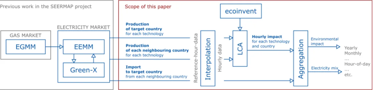
The assessment builds on the linking of an electricity market model with life cycle assessment for the evaluation of the envi- ronmental impact of electricity supply from the grid (Fig. 1). This will be used for assessing the long-term evolution of the electricity system and the variations in the environmental impact on an hourly, daily, monthly and seasonal basis. The output of the market model (electricity production and import-export amounts) is pro- cessed to generate the hourly data. The environmental impact is calculated for every hour, then several aggregation methods are applied to evaluate the impact and the corresponding electricity mix on different timescales. The market model, the environmental impact assessment and the linking is described in more detail in the following chapters. First results based on the simplified version of this linked model were published in (Kiss et al., 2019), since then major updates have been introduced in the methodology.

2.1. Electricity market model

Methodology and assumptions used for electricity market modelling are summarised in this section. The forecast for the electricity mix from 2018 to 2050 was done by the interaction of the European Electricity Market Model (EEMM) of the Regional Centre for Energy Policy Research (REKK), and the Green-X model, developed by the Energy Economics Group of the Vienna University

of Technology (for more details on the models, see (Capros et al., 2014;Mez}osi and Szabo, 2016):). The projection was carried out in the framework of the South East Europe Electricity Roadmap (SEERMAP) project (Szabo et al., 2017), and results were used for further calculation for the analysis presented in this article. The aim of the SEERMAP project was to assess the impact of different policy scenarios on power generation investment decisions, focusing mostly on the SEERMAP region (Albania, Bosnia and Herzegovina, Bulgaria, Greece, Serbia, North Macedonia, Kosovo,¹Montenegro and Romania), but modelling the whole European electricity sys- tem. The forecasts are the result of an iteration between the two models, which ensures that wholesale electricity prices, profile- based renewable energy (RES) market values and capacities converge between EEMM and Green-X.

EEMM is a partial equilibrium microeconomic (supply-demand) model. It assumes a fully liberalised electricity market and perfect competition in all modelled countries, electricity generation and cross border capacities are used/allocated without gaming or ca- pacity withholding. In every country, the model calculates the merit-order curve, assuming all production units offer their elec- tricity on a marginal-cost basis. Supply includes imports as well, with given capacity constraints. EEMM includes 3400 power plant units in a total of 41 markets, including the EU, Western Balkans and other EU neighbouring countries. Each country is a single node in the model, with 104 interconnectors between them.

The EEMM models 90 representative hours of every year.

Reference hours are specified with respect to different supply and demand conditions, considering yearly and daily seasonality. This way production of intermittent renewable capacities (wind, solar and hydro) and of cogeneration fossil fuelled units can be modelled precisely. Hours are grouped in a way that the difference between the original and the modelled load curve is minimised. One important limitation of this approach is that neither the stochastic nature of RES generation, nor ramp-up costs and constraints are considered in the modelling. In this paper, the results for all 8760 hours of the year are interpolated from the reference hours.

Based on short and medium term official national plans and market information, already allocated investment in new fossil- fuel-based generation capacity is included exogenously in the model. On top of that, the model “builds” new fossil-fuel-based capacities endogenously if the investment is economically viable:

it is assumed that power plant operators estimate future costs and make investment decisions based exclusively on expected profit- ability. Different weighted average cost of capital (WACC) values are included in the modelling for every country. Only income from the wholesale market is included in the calculation, the reserve market and balancing market is not modelled.

Fig. 1.Flowchart of the methodology and the link to economic model from the SEERMAP project based on (Szabo et al., 2017).

1 This designation is without prejudice to position on status, and it is in line with UNSCR 1244 and the ICJ Opinion on the Kosovo declaration of independence.

The main inputs of the model are CO2quota and fossil fuel prices (oil, coal, lignite, natural gas), from which forecasts for the latter are provided by REKK’s European Gas Market Model (EGMM) (Kiss et al., 2016) for each country and for each year up to 2050. Year- on-year increase of demand in different countries is based on PRIMES (Capros et al., 2016) data for the EU, while in case of non-EU countries information from national experts included in the SEERMAP project is used.

The model is conservative with respect to technological de- velopments, such as battery storage, fusion, etc., therefore no major technological breakthrough is assumed in the given time frame.

Demand side management (DSM), however, is taken into account, assuming 5% of total daily load is to be shifted by 2050. Con- sumption is transferred from hours with the highest residual load (total demand e0 marginal cost generation), to hours with the lowest residual load, reflecting the fact that prices correlate better with residual load than with total load in case of high RES penetration.

The Green-X model complements the EEMM with more detailed information on renewable electricity potential, policies, geographical distribution and capacities. The model uses a detailed methodology for calculating renewable energy potential for all technologies (using GIS-based information and technology char- acteristics on one hand, and land use and power grid constraints on the other). The limits of renewable scale up is captured by a tech- nology diffusion curve. This accounts for non-market barriers to renewables and assumes learning curves (increasing global RES penetration results in decreasing costs over time). The same way as it is included in the EEMM, Green-X applies different cost of capital in each country and for each technology, by using country and technology specific WACC values. RES investment is endogenously calculated by the Green-X model, taking into account different policy assumptions and all above mentioned parameters.

While in the existing approaches in most cases the used energy system models minimize the discounted sum of energy system costs, EEMM maximizes total welfare of market participants.

2.2. Environmental impact assessment

Standards provide a general framework for conducting an LCA study (ISO 14040, 2006;ISO 14044, 2006). The four phases of LCA are 1) the goal and scope definition, 2) inventory analysis, 3) impact assessment and 4) interpretation.

The functional unit for the calculation is 1 MWh of low-voltage electricity supply at grid. The product system includes the elec- tricity generation technologies of a country, imports and the infrastructure as well as the transmission and distribution systems’ losses. The spatial boundary includes the assessed country and its neighbours. Imports are modelled as the production mix of the adjacent countries (excluding their imports), based on the M2 model described in (Itten et al., 2014). The model assumes that the composition of the exported electricity is the same as supply to the grid. The production mix of a country and the neighbouring countries is provided by the EEMM model. The temporal boundary can be adjusted to the scope of the study and may include the current situation and long-term scenarios with different resolu- tions (hourly to yearly averages).

The calculation is based on the ecoinvent v3.2 database. For allocation, the cut-off system model is applied (Wernet et al., 2016).

The link between the ecoinvent database and the EEMM model output is further explained in the following chapter. Results are assessed for Cumulative Energy Demand (CED), CML (6 most important indicators described in (EN 15978, 2011) and (Bruijn

et al., 2002)), and ReCiPe Endpoint impact categories (Huijbregts et al., 2016) (see Table 1). The first two impact assessment methods are commonly used in LCA practice. ReCiPe introduces the additional feature of a weighted total indicator, that expresses all environmental impacts in three end-point categories, whilst still relying on the principles of thefirst two. In this paper, the results of the Global Warming Potential (Climate changeeGWP 100a/GWP) are analysed in more detail. The assessment was carried out in the OpenLCA software.

2.3. Model linking

When analysing differentfields and sectors, the application of one integrated, comprehensive model many times leads to highly complicated problems and models, with very long calculation times and not always existing solutions. A possible approach to avoid these undesirable situations is the combination of differentesuf- ficiently detailed, but still not too complicated - sub-models. One typical example is the linking of macroeconomic models (typically top-down computable general equilibrium: CGE models) with sector specific (e.g. energy) models (Helgesen and Tomasgard, 2018). Many examples of model linking approaches in the litera- ture in this particularfield can be found.

Model linking can be classified in different ways:Wene (1996)is among the first ones applying two categories: soft-linking and hard-linking. This terminology is now commonly used in the literature by others as well. The more recent paper ofHolz et al.

(2016) summarises modelling approaches. They apply different categories both for models (e.g. top-down and bottom-up models, CGE or partial equilibrium models), and for model linking (soft- linking, hard-linking), including examples for all approaches. In this sense, soft-linking means only information transfer, thus the output of one model is used as an input for the other. In case of hard-linking, the level of integration is higher, at least information transfer is an integral part of the modelling itself.B€ohringer and Rutherford (2008)define three levels of integration: coupling of models; choosing one of the models as the main one and com- plementing it with a reduced form of the other; directly combining the models as mixed complementarity problems. This third solu- tion usually needs to apply simplifications and includes less detailed representation of the system to arrive at a solvable problem.

Soft-linking is probably the most commonly used approach, typical for combining energy-sector specific and other models. In the article ofdel Granado et al. (2017), soft-linkage methodology is applied to two sector-specific models (RAMONA for gas sector and EMPIRE for the electricity sector) to assess the interaction between gas and electricity markets, focusing on the possible changes induced by increased renewable penetration.Krook-Riekkola et al.

(2017)apply soft-linking of a CGE and an energy system model to obtain a more precise modelling framework for the Swedish energy and climate planning. Their results confirm that more precise es- timations can be generated with model linking, as it can capture interactions between sectors.

In this paper, soft-linking between the electricity market model and life-cycle assessment is applied. The EEMM model is used to forecast the composition of the energy production in an hourly resolution, then life-cycle assessment is carried out based on the outputs of the EEMM model. The electricity mix is generated based on the share of electricity generation technologies.

3. Case study

The model is illustrated on the example of the Hungarian grid electricity supply system. The Hungarian case is relevant, as the electricity supply heavily relies on fossil fuels, but substantial decarbonisation is expected soon. Also, it is a relatively small country with a high interconnection capacity where a considerable ratio of the electricity supply is imported. The appropriate model- ling of tradeflows is hence very important.

3.1. Scope of the assessment

The functional unit of the assessment is 1 MWh of low-voltage electricity supply at grid. The product system for the assessment includes the electricity generation technologies of Hungary, im- ports, infrastructure and losses. In the EEMM thefirst modelled year is 2018. The modelled supply mix is the following: 37% nuclear power, 12% lignite power, 13% natural gas power, 8% renewable sources and 30% import, that only slightly differs from the actual 2018 values. The temporal boundary is the present situation and three future scenarios until 2050 (as described in 3.2). Life cycle stages from cradle to grid are considered. The spatial boundary includes Hungary and the neighbouring countries Austria, Slovakia, Croatia, Romania, Serbia, Ukraine and Slovenia.Table 2shows the categories used by the EEMM model, and the corresponding ecoinvent flows used in the LCA in case of Hungary. Different technologies are available in Hungary and the neighbouring countries. The ecoinvent database usually provides country- specific processes, but only for those technologies that are currently available. Since the economic model also considers new power plants in the future, they are modelled as generic (rest-of- the-world, RoW) processes or the dataset of a similar country is used. The country code of the appliedflows is indicated inTable 2.

In some cases, the EEMM model distinguishes between different technologies, where no appropriate process can be found in the ecoinvent database (such as combined cycle and open cycle gas turbines). In this case, the production is added to the technologi- cally closest category (marked as“sum”in the table). In other cases, ecoinvent provides more detailed processes than the EEMM model, here the standard share based on the original ecoinvent mix is used to divide the output of the EEMM model (marked as“rate”in the table).

It should be mentioned that nuclear-based generation is included in the modelling exogenously, based on the latest avail- able information on the decommissioning and commissioning date of“Paks 1”(existing) and“Paks 2”(planned) nuclear power plants.

According to this information, the two power plants (or at least some of their blocks) will operate in parallel between 2030 and

2036. Also the closure of Matra lignite power plant is included in the modelling exogenously, and assumed to happen by 2025.

Some technologies offer combined heat and power generation (CHP), which can be relevant in regions where district heating is widely used: in Hungary, the share of district heating from all heating technologies is around 17% (Hungarian Energy and Public Utility Regulatory Authority, 2016). The allocation of environ- mental impact for co-production (heat and power cogeneration) is a well-known issue in LCA. From both the economic and the environmental aspect, the most important question is which product (heat or power) is the main driver. If heat, then electricity is very cheap as a by-product, so it lies at the very bottom of the merit order. On the other hand, if electricity is the main driver, then CHP plants are usually near the top of the merit order, because the relative cost for power generation is high and depends much on the used technology. This is especially important when the marginal technology is assessed. In this study, the power generated by CHP plants is mainly driven by the heat demand, so it is defined exog- enously based on statistical data.

3.2. Description of the future scenarios

Using data for a specific year may considerably reduce the reliability and the applicability of the results to describe the situ- ation for other years. However, future scenarios involve high un- certainties due to competing technologies and climate policies. The uncertainty may be addressed by comparing several scenarios in a sensitivity analysis. In the SEERMAP project three different sce- narios were established, which are also used for the purposes of this analysis. The main characteristics of the scenarios are sum- marised inTable 3.

The“Decarbon”scenario includes an emission reduction target of 94% for 2050ecompared to 1990 emission levels -, in line with the long-term indicative EU emission reduction goal of 93e99% for the electricity sector as a whole (European Commission, 2011). In this set-up only power plants with a Final Investment Decision (FID) are included in the modelling exogenously, all other new fossil fuelled capacities are added by the model endogenously. This re- flects the more serious commitment to climate protection policies, which goes hand in hand with more ambitious deployment of RES capacities from the beginning of the modelled period.

The“Delayed”scenario represents a later reaction from policy makers in thefield of climate policy. It involves the realisation of current fossil investments included in national plans, followed by a change in policy direction from 2035 onwards. This means that the above targets are in place for 2050, however the investment in RES capacities is less intensive in thefirst 15e20 years (only continu- ation of current RES support policies is assumed), and then support Table 1

Life cycle impact assessment methods and the environmental indicators used in this paper.

LCIA method Indicators Unit

Cumulative Energy Demand Non-renewable energy resources MJ-eq.

Renewable energy resources MJ-eq.

Total MJ-eq.

CML 2001 Acidification potential - average European - AP kg SO2-Eq.

Climate change - GWP 100a kg CO2-Eq.

Depletion of abiotic resources - ADP kg antimony-Eq.

Eutrophication potential - average European - EP kg NOx-Eq.

Photochemical oxidation (summer smog) - high NOx POCP kg ethylene-Eq.

Stratospheric ozone depletion - ODP steady state kg CFC-11-Eq.

ReCiPe Endpoint (H, A) Ecosystem quality - total Points

Resources - total Points

Human health - total Points

is increased sharply from 2035 to reach the mentioned CO₂emis- sion reduction target.

The “No target” scenario sets no long-term goal for carbon- dioxide emission reduction, neither for the SEERMAP region, nor for the rest of the EU. In line with this, it involves the realisation of all fossil-based investments indicated in national plans, and sup- port for renewable energy is phased out after 2025. It is important to note that the“No target”scenario does not serve as a business as usual or„reference”case. Comparing the results of the no target and the other two scenarios can give us hints on what target setting offers.

Targets are set for the EU and for the SEERMAP region as a whole, thus investments are realised in the country with the most favourable conditions: as presented above, models take into ac- count WACC levels (including country-specific, support scheme specific and technology specific risks), and technology diffusion curves when choosing the next site to be built to reach the targets.

This leads to cost-minimisation, as the cheapest investments (in a sense ofV/MWh) are realisedfirst: e.g. a PV plant is“cheaper”if it can produce more electricity - as a result of better solar radiation -

for the same investment cost, or can produce as much electricity for a lower cost, as a result of a lower WACC.

4. Results and discussion

In the following, the variation in the environmental impact of 1 MWh low-voltage electricity supply from the grid is analysed for the case study of Hungary. First of all, the long-term evolution of the electricity system is evaluated on a yearly basis. Then, standard statistical assessment is carried out on the hourly resolution data in specific years. The intra-annual behaviour is assessed for monthly and seasonal variations and within a day. Finally, the limitations of the model are described. Due to the large amount of data, only selected results are presented here,figures and tables for all sce- narios and indicators are found in the Annex.

4.1. The current electricity mix

The average Global Warming Potential and the non-renewable Cumulative Energy Demand of the Hungarian electricity mix is Table 2

Electricity production technologies of the EEMM model and the corresponding ecoinventflows and country codes. (*sum: summarised production of the different tech- nologies, rate: production divided based on default ecoinvent share in the corresponding country) (CHP: combined heat and power generation, CCGT: combined cycle gas turbine, OCGT: open cycle gas turbine, RoW: rest of the world).

EEMM category

CHP func*ecoinventflow Hungary

- HU

Austria - AT

Slovakia - SK

Croatia - HR

Romania - RO

Serbia - RS

Ukraine - UA

Slovenia - SI

nuclear e e electricity production, nuclear, pressure water reactor HU RoW SK RoW e RoW UA SI

electricity production, nuclear, pressure water reactor, heavy water moderated

e e e e RO e e e

lignite e e electricity production, lignite HU RoW RoW HR RO RS RoW SI

yes e heat and power co-generation, lignite SK RoW SK RoW RoW RoW RoW SI

natural gas CCGT

e sum electricity production, natural gas, combined cycle power plant HU AT SK HR RoW RoW UA RoW natural gas

OCGT natural gas

thermal

e electricity production, natural gas, conventional power plant HU AT SK HR RO RoW UA SI natural gas

CCGT

yes e heat and power co-generation, natural gas, combined cycle power plant, 400 MW electrical

HU AT SK HR RO RoW RoW RoW

coal e e electricity production, hard coal AT AT RoW HR RoW RoW UA RoW

yes e heat and power co-generation, hard coal SK AT SK RoW RoW RoW RoW RoW

wind e rate electricity production, wind, 1e3 MW turbine, onshore HU AT e HR RO RoW UA RoW

electricity production, wind,<1 MW turbine, onshore HU AT SK HR RO e UA e

electricity production, wind,>3 MW turbine, onshore HU AT e e RO e UA e

biomass e rate heat and power co-generation, wood chips, 6667 kW, state-of- the-art 2014

HU AT SK e RO e e SI

heat and power co-generation, wood chips, 6667 kW e e e HR e UA e

heat and power co-generation, biogas, gas engine HU AT SK HR RO RS SI

PV e e electricity production, photovoltaic, 570kWp open ground installation, multi-Si

ES ES ES ES ES ES ES ES

run-of-river e e electricity production, hydro, run-of-river HU AT SK HR RO RS UA SI

storage e e electricity production, hydro, reservoir, non-alpine region SK e SK e RoW e RoW RoW

electricity production, hydro, reservoir, alpine region e AT e HR e RS e e

heavy fuel oile sum electricity production, oil HU AT SK HR RO RoW UA SI

Light fuel oil e

geothermal e e electricity production, deep geothermal RoW AT RoW RoW RoW RoW RoW RoW

pumped storage

e e electricity production, hydro, pumped storage SK AT SK HR RO RS UA SI

Table 3

Summary of analysed scenarios in the SEERMAP report (source:Szabo et al., 2017):

Decarbon Delayed No Target

CO2target 94% reduction 94% reduction No target

Fossil plants Only FID From national plans From national plans

RES investments More ambitious RES deployment from 2020 to reach the 2050 target

Continuation of current policies till 2035, and then high uptake

Phase out of support after 2025

Shared assumptions of the 3 scenarios

demand, CO2and fossil fuel prices, gas infrastructure, WACC, NTCs

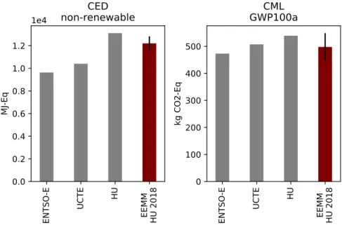
498 kg CO2-eq/MWh and 12 205 MJ-eq/MWh in the EEMM model in 2018. The standard deviation of the mix is 51 kg CO₂-eq/MWh for GWP and 617 MJ-eq/MWh for CED. These values are compared with the available datasets in ecoinvent v3.2, which are generally applied in standard LCA (Fig. 2). The values in ecoinvent are in a similar range but slightly higher for Hungary (539 kg CO2-eq and 13 107 MJ-eq), however, please note that they are based on energy statistics from 2012.

As a reference, the impact of the Hungarian ecoinvent mix is compared to the average of the ENTSO-E network (European Network of Transmission System Operators) representing 43 elec- tricity transmission system operators from 36 countries across Europe and the average for the UCTE countries (continental Europe without Nordic countries) available in ecoinvent. The GWP of the Hungarian ecoinvent mix is higher than the UCTE average (507 kg CO2-eq) and the ENTSO-E (473 kg CO2-eq). For CED, the values for Hungary are much higher than for the UCTE and for the ENTSO-E countries. This can be explained by the relatively high share of nuclear power plants in Hungary, which have a low contribution to GWP, but a high contribution to CED.

4.2. Long-term variation

The total demand is expected to grow by about 26% until 2050 in all scenarios in the EEMM model, represented by a dotted line in Fig. 3a and Annex,Fig. A1.1-3. The growth rate is included exoge- nously in the EEMM. The supply includes the sum of the production and the imports, minus the exports. In the“Decarbon”scenario, it is visible that the penetration of renewables increases, whilst the share of fossil fuels decreases until 2050 (Fig. 3a). Renewable-based generation comes mostly from wind energy, while PV and hydro combined remains under 3% in all years. The nuclear share remains about 35% until the end of the modelled period, except when Paks 1 and Paks 2 will produce electricity in parallel. In these years, Hungary’s import need goes down to around 20%. Otherwise, the import component matches the current rate of around 30e40%.

Fig. 3b shows the evolution of the environmental impact of 1 MWh electricity mix over the analysed period until 2050 for GWP.

Despite the 26% growth in demand, an 87% reduction in the envi- ronmental impact is observed in the long-term compared to 2018, which is due to the fact that in this scenario the 2050 decarbon- isation goals are met. After 2025, the shutdown of lignite power plants reduces the impact significantly. Most of the remaining impact is due to the use of natural gas. Nuclear power does not contribute much to GHG emissions in its life cycle; however, it contributes much more to the CED non-renewable impact category (see Annex A1.1). The long-term change in the environmental impact is presented inTable 4for selected other indicators. In most of the categories, the reduction is 80e87% compared to 2018, except for the non-renewable CED and ODP where only about 36%

and 10% cut is foreseen, respectively.

The“Delayed”scenario is similar to the Decarbon scenario, but the uptake of renewables is slower and hence also the reduction in the environmental impacts (see Annex A1.2). In this scenario, nat- ural gas disappears from the system entirely by 2050. This is due to the need for a huge uptake of RES capacities at the end of the period, thus renewables crowd out natural gas production entirely.

This results in slightly lower environmental impacts in 2050 than in the Decarbon scenario.

The“No target”scenario leads to a far lower renewable share than the other two (see Annex A1.3). Lignite disappears by 2030 in this scenario, too. Natural-gas-based production accounts for 40%

of total energy consumption in 2050. The high share of natural gas is because there is no constraint on GHG emissions. As a result, GWP decreases by only about 30% and non-renewable CED by 9% by 2050, which isn’t as radical as in the other two scenarios. The cut in acidification, eutrophication and photochemical oxidation is still significant (73%, 71% and 50%, respectively).

In all three scenarios, the share of traded electricity (import and export) is relatively high throughout the analysed period, but the related environmental impact decreases (86%,89% and51% in the three scenarios respectively in 2050 in comparison to 2018 for GWP), because of the development of power generation in the neighbouring countries.

Overall, in the “No target” scenario the expected long-term change compared to the current mix is relatively small in the

Fig. 2.Impact of electricity mix processes of ecoinvent v3.2 (reference year 2012) for CED non-renewable and GWP compared to the EEMM model (reference year 2018). Results correspond to 1 MWh of low voltage electricity. (ENTSO-E: European Network of Transmission System Operators; UCTE: continental Europe without Nordic countries; HU: Hungary, EEMM: European Electricity Market Model).

composition of the electricity mix and in the related environmental impact. The “Delayed” and“Decarbon”scenarios both achieve a large impact reduction in the long run with a similar electricity mix.

Importantly, the EEMM model fulfils the decarbonisation

requirement on the scale of an entire market and not locally. This is acceptable from the global environmental point of view. The extensive international trading of grid electricity should not be omitted in an environmental assessment.

Fig. 3.Long term evolution of the electricity mix for the“Decarbon”scenario a) Production and trade b) Environmental impact based on Global Warming Potential. Country codes for import represent the source country (positive import), or the target country (negative import¼export). The total locally consumed electricity (demand) is displayed with a dotted line.

Table 4

Environmental impact of 1 MWh electricity for 2018 and four corner years in the“Decarbon”scenario based on the selected indicators.

Scenario method indicator unit 2018 2020 2030 2040 2050

Decarbon CED non-renewable MJ-eq. 12 205 12 024 10 979 10 133 7752

renewable MJ-eq. 1140 1209 1481 1582 2473

total MJ-eq. 13 345 13 232 12 460 11 716 10 225

CML acidification potential - average European - AP kg SO2-Eq. 2802 1791 0,853 0809 0,362

climate change - GWP 100a kg CO2-Eq. 497,8 376,9 123,4 153,1 63,7

depletion of abiotic resources - ADP kg antimony-Eq. 3550 2695 0,879 1149 0,419

eutrophication potential - average European - EP kg NOx-Eq. 1292 0,892 0353 0,328 0260

photochemical oxidation (summer smog) - high NOx POCP kg ethylene-Eq. 0,1085 0,0714 0,0387 0,0410 0,0199 stratospheric ozone depletion - ODP steady state kg CFC-11-Eq. 7,32E-05 8,06E-05 9,06E-05 9,14E-05 6,59E-05

ReCiPe ecosystem quality Points 9,04 6,86 2,29 2,81 1,24

human health Points 25,36 20,13 7,55 7,42 3,96

resources Points 16,63 12,90 5,15 6,93 2,96

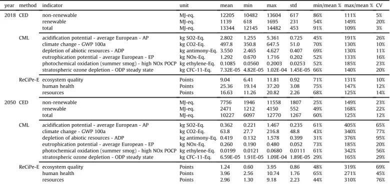
4.3. Intra-annual variation

In order to evaluate the dynamics of the electricity supply, the environmental impact of the electricity mix was analysed with an hourly resolution. The mean, minimum and maximum values as well as the standard deviation (std) and the coefficient of variation (CVestd/mean) are presented inTable 5for the selected indicators for the Decarbon scenario. While the absolute value of the standard deviation for GWP does not increase (51.0 in 2018 and 48.8 in 2050), due to the reduction of the mean (from 497.8 in 2018 to 63.8 in 2050), the coefficient of variation increases from 10% in 2018 to 77%

until 2050. Also, the maximum relative to the mean increases from 130% to 340% for the same indicator.

Even though the reduction in the mean is not that significant for CED as for GWP, CV increases from 5% to 23% for non-renewable energy resources. A large increase of the CV value can also be observed for most of the other CML categories (from 10-26% to 20e95% by 2050) and for ReCiPe, and the same applies to the maximum to mean value. Fig. 4 also supports these results by showing the distribution of the environmental impact (GWP) of 1 MWh electricity in 2018 and 2050 for the“Decarbon”scenario in a box-plot.

The above observations indicate that the intra-annual variation turns out to be more noticeable in future years than today. The high maximum values refer to peak periods regarding environmental impact. The same conclusion can be drawn from the results of the

“Delayed” scenario (see Fig. A2.2 and Table A2 in the Annex), although the values are not that remarkable as for the“Decarbon” scenario. On the other hand, the“No target”scenario (Fig. A2.3 and Table A2in the Annex), shows opposite behavior, in this case a more balanced environmental impact of the electricity supply can be observed, all the way through 2050, just as in 2018.

As the statistical analysis reveals that in some impact categories the hourly impact has a high standard deviation in 2050, next it is examined whether there is a seasonal, monthly, daily or hourly pattern.

4.3.1. Monthly and seasonal variation

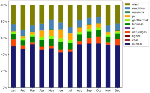
Fig. 5shows the comparison of the monthly average impact to the yearly average in 2050 for the “Decarbon” scenario. A sub- stantial difference can be observed between months. In general, the impact is lower in the summer and higher in the winter, with some deviations, for example November.

Fig. 6shows the share of technologies in the electricity supply (including import electricity). The difference in the environmental impact is mainly explained by the higher share of renewables in the low-impact months (e. g. more solar production in the summer months in comparison to winter, and higher share of run-of-river in spring), however the effect is caused indirectly by reducing the need for gas power. The impact of fossil power in GWP is at least one order higher than of all other sources, so the relative change in the share of fossil energy sources in the mix has high impact on the total. Similar tendencies can be observed in the“Delayed”scenario (Annex Fig. A3.3.1 and A3.3.2). In the current mix and the “No Target” 2050 scenario, the deviations are much lower (Annex Figs. A3.1.1, A3.1.2, A3.4.1 and A3.4.2).

It might be interesting to compare the heating and the non- heating period, for example for the evaluation of electricity use in buildings. The heating season starts usually in mid-October and ends in mid-April in Hungary. However, according to our results, no significant difference can be observed between the averages of these periods (SeeFig. 7and AnnexFig. A4.1-A4.4.)

4.3.2. Variation within a dayepeak and off-peak periods

In Fig. 8 the difference of the hourly impact from the year average is plotted on a heatmap for the year 2050 for the“Decar- bon”scenario to have a better picture on the pattern of daily var- iations in the environmental impact over the entire year. Each column of the heatmap represents one day of the year and each row represents an hour of a day. The colours indicate how much the relative difference is in the environmental impact of that specific hour’s electricity mix to the average of the year. A major difference can be observed between day and night periods. This difference is

Table 5

Statistical metrics of the intra annual variation in the environmental impact of the hourly electricity mix for the“Decarbon”scenario (all values correspond to 1 MWh electricity).

year method indicator unit mean min max std min/mean % max/mean % CV

2018 CED non-renewable MJ-eq. 12205 10482 13604 617 86% 111% 5%

renewable MJ-eq. 1139 618 1695 231 54% 149% 20%

total MJ-eq. 13344 12145 14482 453 91% 109% 3%

CML acidification potential - average European - AP kg SO2-Eq. 2.802 1.255 5.361 0.725 45% 191% 26%

climate change - GWP 100a kg CO2-Eq. 497.8 350.8 647.5 51.0 70% 130% 10%

depletion of abiotic resources - ADP kg antimony-Eq. 3.550 2.465 4.627 0.407 69% 130% 11%

eutrophication potential - average European - EP kg NOx-Eq. 1.292 0.670 1.716 0.202 52% 133% 16%

photochemical oxidation (summer smog) - high NOx POCP kg ethylene-Eq. 0.1085 0.0560 0.2003 0.0253 52% 185% 23%

stratospheric ozone depletion - ODP steady state kg CFC-11-Eq. 7.32E-05 4.82E-05 1.02E-04 1.45E-05 66% 140% 20%

ReCiPe-E ecosystem quality Points 9.04 6.41 11.81 0.92 71% 131% 10%

human health Points 25.36 19.14 37.20 3.08 75% 147% 12%

resources Points 16.63 11.26 20.82 2.26 68% 125% 14%

2050 CED non-renewable MJ-eq. 7756 1946 11558 1807 25% 149% 23%

renewable MJ-eq. 2471 1212 4150 552 49% 168% 22%

total MJ-eq. 10227 6097 12770 1267 60% 125% 12%

CML acidification potential - average European - AP kg SO2-Eq. 0.362 0.221 1.467 0.235 61% 405% 65%

climate change - GWP 100a kg CO2-Eq. 63.8 27.7 216.8 48.8 43% 340% 77%

depletion of abiotic resources - ADP kg antimony-Eq. 0.419 0.132 1.578 0.399 31% 376% 95%

eutrophication potential - average European - EP kg NOx-Eq. 0.260 0.190 0.480 0.052 73% 185% 20%

photochemical oxidation (summer smog) - high NOx POCP kg ethylene-Eq. 0.0199 0.0121 0.0680 0.0111 61% 342% 56%

stratospheric ozone depletion - ODP steady state kg CFC-11-Eq. 6.59E-05 1.91E-05 1.09E-04 1.89E-05 29% 165% 29%

ReCiPe-E ecosystem quality Points 1.24 0.60 3.95 0.86 48% 319% 69%

human health Points 3.96 2.56 10.74 1.76 65% 271% 45%

resources Points 2.96 1.30 9.18 2.23 44% 310% 76%

bigger in the summer season where the hours between 21:00 and 1:00 represent the environmental peak, while in the winter period a less intensive but longer peak is observed (from 18:00 to 1:00).

This is mainly the result of the different availability of PV produc- tion in day and night hours and in summer and winter. Currently, the environmental impact is also slightly lower during the day and in the summer, but the deviations are much lower (AnnexFig. A5.1).

The use of off-peak electricity is often promoted by suppliers with special tariffs based on historical observation of demand.

Legislation also often supports the use of off-peak electricity, which helps to reduce peak load in the network and so decrease the intra- day variation in demand. However, the variation in the environ- mental impact associated with the electricity does not necessarily correlate with demand.

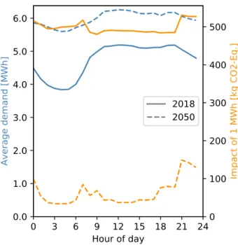
Fig. 9shows the average distribution of the demand within a day parallel to the corresponding environmental impact. For each hour of the day, the average demand is calculated over the entire year, and the environmental impact is derived from the similarly aver- aged electricity mix. The environmental impact shows opposite behaviour to demand both in 2018 and 2050. High periods of de- Fig. 4.Box plot of the environmental impact (in GWP) of the hourly resolution electricity mix for 2018 and 2050,“Decarbon”scenario.

Fig. 5.Average environmental impact (in GWP) of the electricity mix in each month for year 2050 compared to the year average,“Decarbon”scenario.

Fig. 6.Composition of the electricity mix (including import) in each month for year 2050“Decarbon”scenario.

mand can be observed during daylight hours and low at night, while there is a peak in environmental load in the late evening. This means that the environmental impact of the demand peak period is definitely lower than that of the off-peak period, which is against the intuition that peak hours are served by badly performing low efficiency power plants.

The reason is again the share of renewables in the supply mix.

Fig. 10 shows the composition of the production including the imported electricity for a typical summer day in 2050. The high penetration and the daily periodicity of renewable sources is visible. The high impact is observed in the late evening hours, when the demand is still relatively high, but far less renewable energy is available (no PV production). The rest of the demand is served by the only remaining fossil based technology, natural gas powered plants. These power plants are still needed in future scenarios to satisfy the demand when renewable power is not enough, and nuclear plants cannot intervene so quickly.

In the current situation (high share of fossil power) electricity

suppliers put effort into driving away consumption from peak pe- riods, which is beneficial from a system management point of view.

The above observations show that this is disadvantageous consid- ering the environmental impact in Hungary. However, in the future, demand response will offer the opportunity to better match the supply of cheap and low-impact renewable energy.

The high variation is further influenced by the high amount of imported and exported electricity in Hungary. By 2050, the composition of the imported electricity includes much more renewable sources (in both decarbonisation scenarios), therefore the environmental impact of the imported energy varies much more during a year than in 2018. This means that in those countries where electricity trade has a high share and plays an important role in demand equalisation, the import and export should not be excluded from the environmental assessment of the electricity mix.

Although the figures presented above correspond to the

“Decarbon”scenario, most of the conclusions are also true for the

“Delayed”scenario (Figs. A5.3, A6.2, A7.2, A7.3andTable A4). On the Fig. 7.Average environmental impact (in GWP) of the electricity mix in the heating (15th Octe15th April) and the non-heating season for year 2050 compared to the year average,

“Decarbon”scenario (left) and the corresponding composition of the electricity mix (including import) (right).

Fig. 8.Heatmap of the deviation of the hourly impact (in GWP) of 1 MWh electricity from the year average in 2050,“Decarbon”scenario.

other hand, the“No target”scenario is much closer to the current situation (Figs. A5.4, A6.3, A7.4, A7.5andTable A4), where a much lower variation can be observed in the environmental impact mainly because of the low share of renewable energy resources.

4.4. Limitations of the study

An important limitation of our approach is that the EEMM model calculates the electricity mix for 90 reference hours, and results for all 8760 hours are interpolated from these results. The EEMM model uses reference hours to optimize calculation time and

the clustering is optimized based on historical statistical data of the electricity demand. Because of this, the distribution pattern of the demand within a year can only be changed to the extent of the assumed DSM. This leads to a slight distortion in the hourly results, that might increase the further we look ahead in time, as these 90 hours might represent less accurately the same hours in 2050 than they do in 2020. Even if we model all hours of the year, gen- eration of variable renewables, such as wind, solar and run-of-river hydro may vary depending on the weather conditions. This adds unpredictable uncertainties and variations in the input data.

In the soft-linking of the models, some limitations had to be introduced. An increase in the efficiency of the power plants over the years is considered in the economic model, but not in the LCA.

No major technological breakthrough is considered either in the economic or in the environmental model, but the technological learning effects are included in the EEMM and GREEN-X. (Although carbon capture and storage potential has been modelled in the economic model, its effect turned out not to be relevant for the case study).

The modelling of import as the production mix of the exporting country may distort the results in case of“transit”countries that have high amount of import from one neighbour and export to another at the same time.

The use of hourly environmental data may provide more accu- rate results for specific products or processes compared to yearly average data. However, it will increase the complexity of the assessment.

5. Conclusions

In this paper, the linking of an economic electricity market model with life cycle assessment was presented. The model ac- counts for the variation in both local production and import-export by including the production of neighbouring countries and the amount of traded electricity on an hourly resolution. This model can be applied to assess the intra-annual variation of the environ- mental impact today and in future years as well. As the market model has a European scope, it is possible to analyse any European countries with the method developed here.

Three different future policy scenarios were analysed in order to Fig. 9.Average demand distribution within a day and average environmental impact

(in GWP) of the corresponding electricity mix for the years 2018 (left) and 2050 (right),

“Decarbon”scenario.

Fig. 10.Composition of the electricity mix (including import) in a typical summer day of year 2050 in the“Decarbon”scenario.