Potential effects of market power in Hungarian solar boom

(1)

Potential effects of market power in Hungarian solar boom

^*

Oliv er Hortay

^a^,^b^,^*

, Attila A. Víg

^c

aBudapest University of Technology and Economics, Department of Environmental Economics, M}uegyetem rkp. 3, 1111, Budapest, Hungary

bSzazadveg Economic Research Institute, Hidegkuti Nandor u. 8-10, 1037, Budapest, Hungary

cCorvinus University of Budapest, Department of Finance, F}ovam ter 8., 1093, Budapest, Hungary

a r t i c l e i n f o

Article history:

Received 10 January 2020 Received in revised form 24 July 2020

Accepted 14 September 2020 Available online 17 September 2020

Keywords:

Renewable energy Cournot competition Floating premium subsidy Ownership structure Solar production

a b s t r a c t

The Hungarian Government intends to increase the photovoltaic capacities installed in the country sixfold between 2020 and 2030. New investment is encouraged by aﬂoating premium support system in which producers sell electricity on the market and can thus have a direct impact on prices. This article simulates hourly volumes and price data in a Cournot equilibrium model, taking into account the technical and economic characteristics of electricity producers. The model was calibrated with Hungarian data from 2019 and then a theoretical year of 2030 was simulated at different market concentrations. The results show that if prices are above premium levels, operators may reduce their production and thus increase prices as market concentration increases. This phenomenon could dampen the expected price reduction despite the increasing penetration of zero marginal cost solar capacities and threaten the country’s renewable production commitments for 2030. Below the premium level, the effect of market power does not prevail, and prices can nose-dive. In this case, renewable production targets are achieved, but the state’s premium subsidy payments are signiﬁcantly increased. Sensitivity analysis shows that the amount of new photovoltaic capacities and increased electricity demand both increase the effects of market power.

1. Introduction

In recent years, the two key objectives of the European Union’s energy policy e the liberalisation and decarbonisation of the electricity market e have been converging. In the past, most Member States provided contractuallyﬁxed feed-in tariffs (FIT) for renewable producers, which have effectively stimulated in- vestments but made a limited contribution to the market integra- tion of these participants [1]. This distortion runs counter to the

liberalisation efforts, and therefore, in 2014 the European Com- mission issued a decision requiring Member States to replace their FIT with feed-in premium (FIP) starting from 2017 [2]. The point of FIP is that producers must sell on the market and receive a premium over the selling price (the choice of the exact premium logic remains a Member State competence). Thus, producers entering the new support system make sales decisions on a market basis, in which strategic behaviour may appear.

Renewable technologies are less sensitive to economies of scale than fossil fuels, creating opportunities for smaller investors to enter the market, which could lead to decentralisation and increased competition [3]. In contrast, non-residential renewable projects often show neither territorial nor market decentralisation.

New capacities are often developed in a concentrated area and ownership structure, in line with the established oligopolistic market structure. Although in the case of weather-dependent renewables, the actual wind strength and sunshine determine the maximum capacity of producers, they can control the amount produced between their minimum and maximum capacity (see for example [4] for solar power plants). Therefore, if renewable producers entering the market become price-makers due to ownership concentration, they may be able to increase their proﬁts by

*This work was supported by the National Research, Development and Inno- vation Fund of Hungary [Funding scheme: Vallalati KFI_16. Project no. KFI_16-1- 2017-0110]; the Ministry of Human Capacities [Higher Education Excellence Pro- gram, Biotechnology research area of the Budapest University of Technology and Economics (BME FIKP-BIO)]; and the Higher Education Institutional Excellence Program of the Ministry of Human Capacities in the framework of the‘Financial and Public Services’research project (NKFIH-1163-10/2019) at Corvinus University of Budapest.].

*Corresponding author. Budapest University of Technology and Economics, Department of Environmental Economics, M}uegyetem Rkp. 3, 1111, Budapest, Hungary.

E-mail addresses: hortay@eik.bme.hu (O. Hortay),attila.vig@uni-corvinus.hu (A.A. Víg).

Contents lists available atScienceDirect

Energy

j o u r n a l h o m e p a g e :w w w . e l s e v i e r . c o m / l o c a t e / e n e r g y

https://doi.org/10.1016/j.energy.2020.118857

(2)

restraining some of their production. Thus, their revenues can be higher if they limit their production and sell for a high market price as opposed to producing at full capacity. As EU member states devote significantfinancial and intellectual resources to increase the penetration of renewable energy sources, it is in the com- munity’s best interest to understand how such distortions can reduce the efficiency of resource utilisation, and raise prices.

One of the most common approaches in the literature to study oligopolistic behaviour between electricity producers is the Cour- not competition framework [5]. Previously, a few articles examined the impact of renewable producers and government interventions on the operation of deregulated electricity markets. The results showed that without subsidies, the effect of increasing renewable capacities on prices depends on the ownership structure: an increase in market concentration can increase the expected value of prices [6] and volatility [7]. Nevertheless, subsidies have an impact on the behaviour of firms. Producers in the FIT system are not characterised by strategic behaviour and are therefore independent of Cournot competition [8]. Thus, in the FIT, renewables displace conventional power plants [9]. In contrast, Dressler [10] compared in a theoretical framework thefirms’strategic behaviour in the FIP and the FIT systems and found that strategic behaviour appears in the former, and curtailed production may jeopardize countries’ renewable energy commitments. However, to better understand the potential strategic behaviour of FIP-supported renewable producers, Dressler’s theoreticalfindings need to be examined in a complex market environment.

The main contribution of this article is to be theﬁrst to examine the strategic behaviour of FIP-supported photovoltaic producers by taking into account the real ownership structure and market pro- cesses of a country. Currently, only FIT-supported power plants operate in Hungary, but the government aims to achieve its 2030 policy goals primarily with new FIP-supported photovoltaic capacities [11]. This paper examines the impact that increased market concentration of new producers may have on market prices and the achievement of renewable energy targets. To this end, a dynamic, multi-stakeholder Cournot model was calibrated, based on 2019 Hungarian power plant portfolio, ownership structure, technological constraints, fuel prices and weather data. Then, the power plant portfolio and electricity demand were modiﬁed based on the Hungarian government’s energy strategy for 2030: FIP-supported

installed photovoltaic capacity was increased by 4000 MW, old fossil power plants were closed, and electricity demand increased by 25% [11]. All other parameters remained unchanged. Newly entering photovoltaic capacities were distributed equally among a varying number of owners, and the simulations were run separately for each owner number. The effect of market power was illustrated by a decrease in the volume of monthly solar production and an increase in average market prices. Finally, a sensitivity analysis was performed on electricity demand, installed photovoltaic capacity, and FIP level.

The structure of the article is as follows. Section2describes the applied methodology: the Cournot model, its assumptions, the data used and its sources. Section3presents the results of the study.

Finally, Section4summarises the main conclusions of the research and future works.

2. Methodology

This section details the Cournot equilibrium model setup, the concept of calibration and data. The general assumptions of the model are detailed in Appendix A. The ﬂowchart for the work performed is shown inFig. 1.

The methodology used consists of three distinct parts: calibration, simulation, and sensitivity analysis. In theﬁrst, the equilibrium model was calibrated on 2019 data. During simulation, the calibrated model was run for the 2030 inputs. Finally, a sensitivity analysis was performed for the key variables.

2.1. Equilibrium model setup

LetIdenote the set of competing power plants withjIj ¼n. The time dimension is indexed byt2T, where eachtrepresents an hour in the electricity market. Each power planti2Iis characterised by its marginal cost of productionc_i_;_t2Rat timet2T and capacity constraints½0;C_i;t3R. Marginal costs vary in time due to fuel cost changes, while capacity constraints are constant for regular power plants but do change for solar plants and wind turbines due to weather effects [10]. The exact calculations for marginal costs and capacity constraints are detailed inAppendix B.

Power planti2Iis also characterised by its up-down gradient Nomenclature

Abbreviations

FIT feed-in tariffs FIP feed-in premium

HEPURA Hungarian Energy and Public Utility Regulatory Authority

MAVIR Mavir Hungarian Transmission System Operator Ltd.

Indices and sets

I set of competing power plants i competing power plant index n number of competing power plants t time index, h

A_i_;_t ¼ a_i_;_t;a_i_;_t

action set (interval deﬁned by boundaries) of plantiat timet, MWh

Parameters and constants

c_i_;_t marginal cost power plantiat timet,V$MWh¹

C_i;t maximum theoretical capacity of plantiat timet, MWh

g_i up-down gradient of planti, MW F premium level for FIP producers q_0;t exogenous electricity production Variables and functions

q_i_;_t electricity production of plantiat timet, MWh Pt model price at timet

Qt sum of all production at timet, MWh

at the constant parameter of the afﬁne inverse demand function at timet

rt the slope parameter of the afﬁne inverse demand function at timet

Pi;t proﬁt of plantiat timet,V J Nikaido-Isoda function Z optimum response function

O. Hortay and A.A. Víg Energy 213 (2020) 118857

(3)

g_i>0. The up-down gradient denotes the plant’s speed of adjustment which it is able to change its electricity production from one hour to the next with. Assume that power planti2Iproduces q_i_;_t0 amounts of electricity at time t2T. Then, its action set A_i_;_tþ1¼

a_i;tþ1;a_i_;_tþ1

3½0;C_i_;_tevolves endogenously according to its up-down gradient in the following way:

a_i;tþ1¼max

0;q_i;tg_i

a_i;tþ1¼min

C_i;t;q_i;tþg_i

which in simple terms means that next period production may differ from current output by the adjustment speed of the power plant, but cannot be larger than maximum theoretical capacityC_i_;_t or smaller than minimum theoretical capacity (zero).

The (inverse) demand function is denoted byPtðQtÞfor eacht2 T, whereQt¼q_0;tþP

i2Iq_i;t is the sum of all electricity production, andq₀_;_t is electricity production we consider exogenous.¹Due to

the strong seasonality of electricity consumption, the demand function is assumed to change over time [12]. The afﬁne speciﬁ- cation for the (inverse) demand function is:

PtðQtÞ ¼

a

t

r

tQt

Pi;t denotes the proﬁt function of plantiat timet. The standard form of the function is:

P

i;t

q_i;t;q_i;t

¼

PtðQ_tÞ c_i;t q_i;t; (1) whereq_i;t ¼ ðq0;t;q₁_;_t;…;q_i1;t;…;q_iþ1;t;…;q_n;tÞ2Rⁿ. Expected changes in the premium subsidy system for 2030 mean that the profit function of certain power plants is different toEq. (1). In the floating premium system (FIP), solar power plants also have to compete in the market, but if the market price is below a particular fixed levelF, the state subsidises them up to this level. Thus, the profit function for solar power plants in 2030 becomes:

P

⁰i;t

q_i;t;q_i;t

¼

maxðPtðQtÞ;FÞ c_i;t q_i;t (2) Power plants are competing in the market, and they simultaneously solve their proﬁt maximisation problem, sequentially in time (see for example in Ref. [7,13e15]). This also means that in the setup power plants act in a myopic manner, even though their Fig. 1.Flowchart of the model.

1The single nuclear power plant (Paks) due to its size, renewables producing in the FIT system, and cross-borderﬂows because the investigation of their behaviour is out of the scope of this paper.

(4)

choice of production does have a future effect through their evolving action set due to their up-down gradient. The decision variable of power plants is the amount of electricity they produce:

q_i;t2A_i;t. The model is seeking the production proﬁlesðq_i;t;…;q_n;tÞ 2Rⁿct2Twhich meets the following criteria:

q_i;t2A_i;t ci2I;ct2T and

P

i;t

q_i;t;q_i;t

P

i;t

q0_i;t;q_i;t

cq0_i;t2A_i;t and ci2I;ct2T The model is seeking a sequence of pure Nash equilibria in a market where power plants can choose their production from a closed interval in each period, and their proﬁt function is quadratic.

The equilibrium production vector can be found by applying the relaxation algorithm of Krawczyk and Uryasev [16], which is based on the so-called Nikaido-Isoda [17] function. The algorithm is brieﬂy described below, but a detailed description can be found in Refs. [16]. The time dimension has been neglected. Letq¼ ðq1;…;

qnÞ. The Nikaido-Isoda function J:RⁿRⁿ1R is deﬁned as follows:

J

ðq;q⁰Þ ¼Xⁿ

i¼1

P

iðq_i⁰;q_iÞ

P

iðqÞ

LetA¼A_i…An3Rⁿ. A production vectorq⁺2Ais Nash equilibrium if

maxq2A

J

ðq⁺;qÞ ¼0

The optimum response function (possibly multi-valued) is:

ZðqÞ ¼argmax

q⁰2A

J

ðq;q⁰Þ; q;ZðqÞ2A

Function Z returns² the production vector that is optimal for each power plant in the sense that it maximises their proﬁt if they unilaterally change to it. Letq⁰2Abe aﬁrst estimate for the Nash equilibrium. Let the recursion

q^sþ1¼ ð1

b

sÞq^sþ

b

sZðq^sÞ; s¼0;1;… be such that 0<bs1 andP_∞

s¼0bs¼∞and lims/∞bs ¼0. Then the main theorem of[16]says thatq⁺¼lim_s/∞q^sis a Nash equilibrium. Numerical experimentation proved that bs¼¹_s cs work well for the model.

2.2. Calibration on 2019 data and simulation for 2030

Computations are divided into two parts: calibration (on 2019 data) and then simulationquasi-ceteris paribusfor 2030. Due to this duality, some variables are endogenous during calibration and exogenous during estimation.

The two non-observable quantities of the model described in the previous section are the two parameters (interceptatand slope rt) of the afﬁne demand function. These quantities are calibrated on 2019 data. For the year of 2019, calibration was performed according to two variables: the hourly electricity prices P_t⁺ on the day-ahead market and the total electricity consumptionQ_t⁺. The output of the equilibrium-seeking algorithm is the production vectorqtof power plants andPtprices for eacht. During calibration,

the model looks forðat;rtÞ_t₂_T vectors for which in equilibriumQt

andPt is such that

Q_tQ_t⁺<ε ct2T (3) P_tP_t⁺/min ct2T (4) Thefirst condition means that total production produced by the model should not deviate significantly from the total production observed during the calibration period, demand must be met by supply. The second condition means that the equilibrium price calculated by the model should not deviate significantly from the market price observed during the calibration period.

The calibration is performed in several steps. In theﬁrst step, a grid was taken inrt, the extent of which can vary between the smallest and largest elasticity parameters previously measured according to the literature of Lijesen [18]. At each point of the grid, we look for the vectorða1;…;ajTjÞthat satisfy theﬁrst condition at that constantrt.Q_tis monotone inat, so ifQ_tþε<Q_t⁺in a given t, atwas set to be higher and vice versa. The iteration continues until condition (3) is met, so for everyrin the grid aða1;…;ajTjÞvector is arrived at. In the second step, thertwhich implies an equilibrium pricePtclosest to the observedP⁺_t is selected from the grid, for each t.

During the 2030 simulation, aquasi-ceteris paribusconcept was applied, which means that where credible predictions for input parameters were available in the literature, they were modiﬁed, elsewhere they were assumed to be unchanged. Therefore, the elasticity parameterrt of the demand functions does not change from the one calibrated on 2019 data, while the interceptat is increased by 25% in line with projections of growing power demand for 2030 [11]. The output of these simulations is the quantities producedðqtÞ_t₂_Tby the power plants and the resulting prices ðPtÞ_t2T during the year. Of these, this paper primarily discusses total solar power production and prices in Section3.

2.3. Data

This subsection presents the data used for the calibration, which can be divided into three categories: installed capacity, weather data, and prices. The parameters, that were modiﬁed in the 2030 simulation and that remained unchanged according to thequasi- ceteris paribusapproach, are detailed for each category. The calibration was performed for each hour of the 2019 year. And the output of the 2030 simulation was also a year-long, hourly frequency series.

For the calibration, the current power plant database was reviewed based on the production licenses issued by the Hungarian Energy and Public Utility Regulatory Authority (HEPURA). The main attributes of each unit are the gross installed capacity, the technology and fuel, and the expiration date of the license [19]. Based on HEPURA 2019 data, 7815 MW of active installed capacity was identiﬁed for a total number of 560 units. In the case of fuels;

biogas, biomass, landﬁll gas, sewage gas and waste energy are all treated as biomass. The sum of permanent shortage and surplus was subtracted from the gross installed capacity for each unit, and the resulting available permanent capacity was taken into account as the maximum capacity. The efﬁciency ratios and speeds of adjustment to each block were also assigned from the joint publi- cation of the Mavir Hungarian Transmission System Operator Ltd.

(MAVIR) and HEPURA [20] for large power plants. The small power plants’speciﬁcations were based on the large ones with the same fuel type proportionally. Units with the same owners were linked together, i.e. portfolios were created that represent the players of

2In general, Z is not a function. In this case, however, it is single-valued, so it is a function.

(5)

our model. As a result, the number of players has dropped to 265, with the most signiﬁcant 15 controlling 83% of capacity.

As there is no forecast of future changes in the ownership structure, all units whose license extends to 2030 were considered with the same ownership structure for the 2030 simulations.

Following the quasi-ceteris paribus concept, the existing power plant structure was modiﬁed for the simulation at two points: the closure of obsolete power plants and the entry of new photovoltaic capacities according to the Hungarian energy strategy. Due to the licenses expiring by 2030, it was expected to see the closure of coal capacity and the reduction of natural gas capacity from 3300 MW to 2970 MW. The National Energy and Climate Plan of Hungary [11]

aims to increase the installed capacity with 4000 MW new FIP- supported photovoltaic units; therefore, this amount was added to the simulation. The impact of the concentration was examined with a theoretical approach, in which the new photovoltaic capacities to be built are equally distributed among a variable number of competing ﬁrms. In this case, the increase in the number of producers reduces market concentration and thus leads to increased competition.

Generally, the results of electricity market models are suscep- tible to demand and weather inputs [21]. The source of hourly frequency weather, demand and production data used for calibration was the MAVIR database. In 2019, 29.7% of electricity demand was met by imports, 35.9% from nuclear power, 17.6% from natural gas, 9% from coal, 1.7% from wind, 2.1% from solar and 3.9% from other resources.³Fig. 2shows the monthly distribution of aggregate demand and photovoltaic production. It shows a characteristic difference between winter when heating boosted demand but the low number of hours of sunshine kept photovoltaic production small, and summer (mainly August and September) when relatively low demand was met by large amounts of the photovoltaic output.

In line with the Climate Plan’s [11] forecast, in the 2030

simulation, demand (the parameterat) was increased by 25% every hour. The shape of the wind and solar proﬁles has been left unchanged, but the latter has been scaled with the capacities expected to be installed, thus marking the maximum solar production po- tentials. The hourly output of exogenous actors [22] remained unchanged in the 2030 simulation.

The fuel prices used for calibration were estimated on the basis of the market benchmarks most often used by Hungarian producers [22]. Gas prices were based on average daily prices from the Central Eastern European Gas Exchange spot market and range from 10.51 2MWh¹to 24.89V$MWh¹[23]. Carbon quota prices were based on the European Emission Trading System and range from 18.352 t¹to 29.46V$t¹[24]. Oil prices were proxied by Brent daily prices and range from 55.38$MWh¹to 75.01$$MWh¹[24]. The cost of nuclear fuel was estimated at 3V$MWh¹, coal at 5V$MWh¹ , and biomass at 7V$MWh¹, which were estimated from the 2018 business reports of the companies using these fuels. For model calibration, Hungarian Power Exchange day-ahead electricity market prices were used [25]. As fuel prices are not forecast for 2030, they are unchanged in the simulation.

In 2019, no FIP-supported power plant was operating in Hungary, so it did not have to be taken into account in the calibration. The HEPURA announced the results of theﬁrst FIP tender on March 27, 2020 in which the average premium level of large producers was 64V$MWh¹ [26]. Therefore, this premium level was assumed in the 2030 simulation. Following the simulation, a sensitivity analysis was performed for three parameters: demand growth, the amount of installed photovoltaic capacities, and premium level. The results of the investigation are presented in Section 3.

3. Results and discussion

This section details the results of the benchmark simulation and sensitivity analysis. The 2030 benchmark simulation examined Fig. 2. Monthly distribution of aggregate demand (blue line, left axis) and photovoltaic production (orange line, right axis) in 2019. (For interpretation of the references to colour in thisﬁgure legend, the reader is referred to the Web version of this article.)

3Biomass, biogas, hydro, waste incineration, landﬁll gas and sewage gas.

(6)

how the ownership structure of newly installed FIP-supported photovoltaic producers affects prices and volumes produced. To this end, the model distributed capacity equally among a variable number of owners and generated separate output for each number of owners. Subsequently, a sensitivity analysis was run for three variables (demand, FIP level, amount of new capacity), the results of which showed how the modiﬁcation of the variables affects the restraint of photovoltaic production. Finally, the section discusses the limitations of the results.

3.1. Benchmark simulation

The two main outputs of the benchmark simulation are the volumes produced by power plants and market prices. The model was run for each hour of the year, so the output vector consists of 8760 data points for prices and productions of each competing power plant. For the sake of clarity, the data presented are aggre- gated monthly for the quantities produced and averaged for the prices. Three-dimensional diagrams were used for the represen- tation, showing the number of months on one axis, the number of owners on the other axis, and a decrease in photovoltaic production and an increase in average prices on the third axis. The newly installed capacities were distributed equally among the owners.

The results of the simulations showed that if new photovoltaic capacity is distributed among more than 15 FIP owners, they become price-takers and their market power is eliminated.

Therefore, the results were plotted from 1 to 15 owners. In the model, owners can inﬂuence market prices by reducing their production, soFig. 3shows the ratio of aggregate photovoltaic production to the theoretical maximum.

As a result of the increase in ownership concentration, the effect of market power increases signiﬁcantly, making it increasingly worthwhile for producers to reduce their production in order to increase market prices and thus their proﬁts. The effect is non- linear; thus, if capacities are distributed among one owner

instead of two, the degree of restraint is more than double. In addition to ownership concentration, weather and demand also inﬂuence production decisions (for comparison, seeFig. 2). Irradi- ation determines the maximum useable capacity of photovoltaic producers, and thus their market power, so the restraint of production is the strongest in August, as the 2019 benchmark year also had the highest irradiation. The January results show that high demand will also increase the market power of photovoltaic producers despite their low capacity at the time because demand must be met by supply and solar plants compete mainly with higher marginal cost power plants. The results of September and October also support this phenomenon, as although the theoretically available maximum photovoltaic production was higher in September, the reduction of production was lower due to lower demand. In the case of a single FIP solar plant, yearly photovoltaic production is 26.7% less than production in the perfectly competitive case.

The primary motivation behind the production reduction of price-maker solar power plants is the increase in market prices.

Fig. 4shows that market power can have a signiﬁcant impact on market prices: for a single FIP photovoltaic producer, the simulation resulted in a 29.9% increase in average prices for August. Average prices fall to a lesser extent than the restraint of production, which is because every hour is given equal weight in the average of prices.

In contrast, the theoretical maximum of production of a given hour is the benchmark for the produced quantities. In fact, during the hours when the theoretical maximum of photovoltaic production is high, the rate of price growth may exceed the rate of production restraint. For example, the most signiﬁcant production reduction was simulated at noon on the 5th of September (423 MWh photovoltaic production against 3797 MWh potential) and it resulted in a price ofV126 instead ofV0 in perfect competition. The V0 price in perfect competition is because the Hungarian FIP system does not pay a subsidy if the price is below it. Without this bound, the price may decrease further to the negative area.

Fig. 3.Monthly production by number of FIP solar plants. Monthly production is the ratio of actual production and maximum capacity (taking sunshine-hour into account).

(7)

3.2. Sensitivity analysis

The inputs of the benchmark simulation differ the most from the calibration in the growth of electricity demand, installation of new photovoltaic capacities and introduction of the FIP support system.

Therefore a sensitivity analysis was performed for these three high priority variables. The results of the sensitivity analysis were plotted for effect on production reduction for all three variables because these results are more pronounced than the impact on average prices.

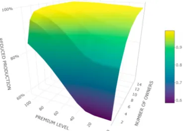
Fig. 5shows the effect of changing the FIP level on production reduction. The benchmark simulation was calculated at the level of 64V$MWh¹ formed in the only auction held in Hungary earlier.

The upper level of the sensitivity analysis range was set at 100 V$MWh¹ based on the results of past German photovoltaic FIP auctions (the previous highest level in April 2015 was 91.7V$MWh¹[27]). 0V$MWh¹ was selected for the lower level because no support can be paid in Hungary below this value.

Fig. 5 shows that as the FIP level increases, the production reduction decreases. This is because if market prices are below the premium level, it does not matter to photovoltaic producers how much the difference between the premium level and the price is.

After all, they will receive revenue corresponding to the premium level per unit of electricity produced. In this case, the actors aim to produce as much electricity as possible. It is only worthwhile for photovoltaic producers to use their market power if prices (even as a result of reduced production) exceed the level of the premium, because only then can they increase their profits. As a result of the change in the premium level, a break can be observed at 40V$MWh¹, which is because prices fall relatively infrequently below this value. In parallel, with the increase in the level of the premium, the reduction in production also flattens out, because prices rarely rise above a certain level. However, the upper level is strongly influenced by ownership concentration, as its growth also increases the frequency of high prices. Within a specific interval (depending on the concentration of ownership), the FIP level has a substantial effect on the reduction in production.

The increase in electricity demand in the benchmark simulation was assumed to be 25%. Still, as this is quite an uncertain estimation, a sensitivity analysis was conducted and is shown inFig. 6. As no other forecast was published for the variable, the study was conducted between 0% to 50% growth extremes.

Although the results of the benchmark simulation showed that an increase in demand raises the phenomenon of production reduction, based on the sensitivity analysis, this is only accurate above a certain level of demand.Fig. 6shows that below a certain level of demand (varying according to ownership concentration), Fig. 4.Monthly average price increase by number of FIP solar plants.

Fig. 5.Dependence of reduced FIP solar production on premium level.

(8)

increasing demand reduces the effect of market power. The reason for this phenomenon is that it is not worthwhile for conventional power plants to produce up to a certain price level because their short-term marginal costs exceed market prices. In this interval, photovoltaic producers have considerable market power and can have a signiﬁcant impact on prices by reducing their production.

However, as demand and thus prices rise, more and more conventional power plants will enter, with which solar power plants will have to compete, and this will reduce their market power. As demand continues to grow, the effect will be reversed, as photovoltaic producers will be needed to maintain the balance of the system, and their market power will thus increase again. This second phase of market power growth is ﬂatter due to greater competition.

Finally, the third variable for which a sensitivity analysis was performed is the amount of new capacity installed. The benchmark simulation assumed 4000 MW of new photovoltaic capacity as it is the ofﬁcial target of current energy policy, but a sensitivity analysis was conducted in the range of 2000 MW to 6000 MW. The results are shown inFig. 7.

Like irradiation, the amount of installed capacity determines the theoretical maximum of production, and thus the market power of producers. If a higher amount of capacity is concentrated in a smaller number of owners, the market power of photovoltaic producers will be greater, and they will thus be more interested in reducing their production. The impact of changes in new capacities is more signiﬁcant if the ownership structure is more concentrated.

3.3. Discussion

The Cournot model built in this paper can handle many complex effects (technological conditions, ownership conditions, system equilibrium condition) arising from the properties of the electricity system, but at the same time, impacts that limit the practical applicability of the results remain. One significant limitation is that while the model only looks at the spot market, in reality, power generators can sell in several different markets. Also, as the in- dustry develops, new markets (such as flexibility markets) may emerge. However, increasing the number of markets requires the implementation of new behavioural patterns of firms, and these further constraints are outside the scope of the article.

Another limitation is that the new owners considered in the

simulation only hold a portfolio of photovoltaic production units. In contrast, it is conceivable that owners will diversify their portfolios and operate other generation and storage technologies in addition to photovoltaic units. In this case, the owners maximise the proﬁt for the entire portfolio, which can lead to different results as if optimised separately for photovoltaic production units. The article does not examine mixed portfolios for new entrants because of the reduction in photovoltaic production in these would also be inﬂu- enced by the composition of the portfolio, which would skew the results.

Finally, the model assumes the short-run marginal cost of photovoltaic producers to be zero because these actors do not have fuel and carbon quota costs. On the one hand, photovoltaic producers can ramp-down their productionﬂexibly and free of charge [4], so the assumption is acceptable. On the other hand, in the spot market, producers have to submit their bids no more than one day before delivery, and the maximum capacity of solar cells cannot be predicted with perfect accuracy in advance. Thus, the unpredict- ability of weather poses a new risk element for photovoltaic producers over conventional power plants, which can be interpreted as a short-run marginal cost, making the assumption questionable.

One of the main difﬁculties in modelling photovoltaic producers’decisions is that while there are large amounts of obser- vations on the use of market power and cost-beneﬁt considerations for conventional power plants, this experience is not yet available for renewable producers. Since, to the best of the authors’knowl- edge, empirical evidence is not yet available to demonstrate that the high ownership concentration of renewable capacities in a market has made individual owners price-makers, potential future effects can only be examined under certain assumptions. However, they are worth addressing ex-ante so that policy can prepare for their eventuality.

4. Conclusion and future work

The Hungarian Government predicts the realisation of a significant amount of FIP-supported new photovoltaic investment by 2030. This article examined in the Cournot framework the potential impact of market power associated with the possible ownership concentration of new capacity on price and on electricity generated by solar panels. Calibration of the model was performed based on Fig. 6.Dependence of reduced FIP solar production on demand growth. Fig. 7.Dependence of reduced FIP solar production on new solar capacity.

(9)

data from 2019, and then the effect of the new units was examined quasi-ceteris paribusby 2030. A sensitivity analysis was performed for the three main inputs that changed compared to the 2019 parameters: growth of electricity demand, FIP support level, and new photovoltaic capacities.

The paper concludes that the potential impact of market power is inﬂuenced by ownership concentration, maximum energy that can be produced by solar panels, electricity demand, the cost structure of conventional power plants, and FIP levels. In the ex- amination of ownership concentration, new capacities were distributed equally among a varying number of companies. The results showed that photovoltaic producers become price-makers in some periods when the number of owners falls below 15. The most substantial inﬂuence can be observed in the monopoly structure, where the amount of annual electricity produced by solar panels is 26.7% lower than in a perfectly competitive market in the benchmark simulation. This results in a 7.92% increase in annual average prices. The higher the available solar cell production is in a period, the higher the market power of the owners, so both the amount of installed capacity and the intensity of irradiation have a positive effect on the production reduction activity. With low demand and price, the market power of photovoltaic producers is high, however, as they begin to rise, producing becomes worthwhile for more and more conventional power plants, thus reducing the market power of photovoltaic power plants. However, at a certain level of demand, the price reaches the short-run marginal cost of the highest controllable power plant in the merit order, so that as market demand increases further, the market power of photovoltaic producers will rise again. Finally, renewable producers should only use their market power if they can push the price above the FIP level. Otherwise, it is worth operating at maximum capacity.

Therefore, the higher the FIP level, the less characteristic the production reduction behaviour will be.

The main policy lesson to draw from the results of the model is that, when designing the rules for allocating subsidies, care must be taken not to create excessive market concentration, as this maye through strategic production reduction ehinder price reduction effects expected from zero marginal cost producers, and endanger the country’s renewable commitments. Sharp price drops below the premium level can be considered favourable by consumers, but on the other hand, they can signiﬁcantly increase public burdens, since premium subsidy payments are much higher in these cases.

An undesirable market distortion effect may diminish the market power of conventional power plants, which may reduce the effec- tive functioning of market mechanisms.

The two most important areas where the model used in the article is worth developing in the future are: refining the behaviour of photovoltaic producers and further implementing the complexity of the electricity market. Exploring the real cost-benefit nexus of decision between not selling and selling the solar energy in the market is an essential condition for making a forecast in addition to determining the potential for market power. Besides, both the interactions between individual electricity markets and the combined optimisation opportunities of different instruments held in companiesâV™portfolios can contribute to a better un- derstanding of the complexity of reality, thus providing a promising direction for further research.

Author contribution

Oliver Hortay: Conceptualization, Investigation, Writing - orig- inal draft Attila A. Víg: Methodology, Software, Validation, Formal analysis, Visualization

Declaration of competing interest

The authors declare that they have no known competing ﬁnancial interests or personal relationships that could have appeared to inﬂuence the work reported in this paper.

Appendix A. Assumptions

The following assumptions were used in the model.

1. There is no co-operation between different electricity companies, meaning that one company only seeks to maximise the proﬁts of its own. This assumption is commonly used in Cournot models, see, for example, the following articles [7]: [13e15].

2. All the country’s supply and demand meet in a single market.

That is, all consumers purchase the electricity they need in the modelled spot market and accordingly, each producer sells there. The reserve market is also not examined, so it does not change the capacity limits of the players. Contreras et al. [28]

uses similar assumption.

3. Producers decide simultaneously on the amount of electricity to be produced for a given period and optimise from period to period independently (see, for example [12]).

4. Cross-borderﬂows, renewables participating in the guaranteed subsidy scheme and the production Paks nuclear power plant are assumed to be exogenous. Paizs [22] used a similar assumption for the Hungarian electricity system.

5. Biomass, biogas, waste incineration, landﬁll gas, and wastewater technologies are treated in a combined manner based on both their technical characteristics and their short-term marginal costs (see, for example [8]).

6. It is assumed that each fuel type will be available to all participants at the same price (see, for example [8]).

7. Because of the quasi-ceteris paribus concept, the current ownership structure is assumed to remain unchanged in 2030 for power plants remaining in the system.

8. As no forecast for FIP levels is available, each participant in the benchmark model produces based on the scale from theﬁrst Hungarian tender [26]. As this is a crucial variable, a sensitivity analysis was performed for the premium level.

9. Under the rules of the Hungarian subsidy system, producers are not entitled to a premium in case of negative prices [29].

Appendix B. Calculations of power plant characteristics

The following parameters characterise eachi2Ipower plant:

fuel_i2fnuclear;naturalGas;oil;sun;wind;water;biomass;coalg denotes the fuel type of the power plant.

globalMaxCap_i>0 denotes the plant’s maximum capacity. Unit of measurement is MWh. (Minimum capacity is assumed to be zero for all power plants.)

hi2ð0;1denotes the efﬁciency ratio of the plant.

g_i>0 denotes the plant’s speed of adjustment. Unit of measurement is MW.

CO2_i0 denotes the plant’s CO₂ emissions. Unit of measurement ist$MWh¹.

While the characteristics of power plants detailed above do not change over time, the model also has a time dimension. Fuel costs, and ultimately the marginal cost of each power plant, change over time. Capacity limits for certain renewable power plants (solar and wind) are also changing due to changing weather conditions. The

(10)

time dimension is indexed byt2T, where a giventdenotes an hour interval. The following data characterise each hour:

P⁺_t 2Rdenotes the spot price of electricity on the DAM market.

Unit of measurement isV$MWh¹.

Q_t⁺>0 denotes net electricity demand, which by deﬁnition is also equal to the sum of all production and import. Unit of measurement is MWh.

cloudt2½0;1denotes the ratio at which solar plants can produce compared to their maximum capacity due to weather. This ratio is trivially zero at night and reaches its highest at or shortly after noon.

windt2½0;1 denotes the ratio at which wind turbines can produce compared to their maximum capacity due to weather.

CO2quota_t>0 denotes the price of CO₂ quota. Unit of measurement isV$t¹.

ðnucPt;coalPt;gasPt;oilPt;sunPt;windPt;waterPt;bioPtÞ2R⁸ denotes the fuel cost of each plant type. Unit of measurement isV

$MWh¹. We note that although the unit of time of the model is an hour, fuel prices usually do not change hourly. For example, the cost of nuclear fuel is assumed to be constant in time.

Furthermore, the cost of renewables is assumed to be constant zero in time. In order to be consistent in the model description, in general, it was allowed all fuel costs to change hourly.

The following power plant characteristics and decision variables are time-dependent:

c_i_;_t>0 denotes the marginal cost of planti2Iat timet2T. Unit of measurement is V$MWh¹ . Marginal cost is calculated by following formula for each fuel type (coal in the example):

c_i;t¼coalPt

h

i

þCO2quota_t,CO2_i

Global capacity constraints change with time for solar and wind power plants due to changing weather conditions. Demon- strating this effect for wind turbines:

C_i;t¼globalMaxCap_i,windt

For other plant typesC_i;t ¼globalMaxCap_i,ct2T.

References

[1] Couture T, Gagnon Y. An analysis of feed-in tariff remuneration models: im- plications for renewable energy investment. Energy Pol 2010;38(2):955e65.

https://doi.org/10.1016/j.enpol.2009.10.047.

[2] European Commission. 2014/C 200/01, Guidelines on State aid for environmental protection and energy 2014-2020. 2014. https://eur-lex.europa.eu/

legal-content/EN/TXT/?uri¼CELEX:52014XC0628(01). [Accessed 25 November 2019].

[3] Hirth L. The market value of variable renewables: the effect of solar wind power variability on their relative price. Energy Econ 2013;38:218e36.

https://doi.org/10.1016/j.eneco.2013.02.004.

[4] Chen X, Du Y, Wen H, Jiang L, Xiao W. Forecasting-based power ramp-rate control strategies for utility-scale PV systems. IEEE Trans Ind Electron 2018;66(3):1862e71.https://doi.org/10.1109/TIE.2018.2840490.

[5] Weron R. Electricity price forecasting: a review of the state-of-the-art with a look into the future. Int J Forecast 2014;30(4):1030e81. https://doi.org/

10.1016/j.ijforecast.2014.08.008.

[6] Ben-Moshe O, Rubin OD. Does wind energy mitigate market power in deregulated electricity markets? Energy 2015;85:511e21. https://doi.org/

10.1016/j.energy.2015.03.069.

[7] Milstein I, Tishler A. Intermittently renewable energy, optimal capacity mix and prices in a deregulated electricity market. Energy Pol 2011;39(7):3922e7.

https://doi.org/10.1016/j.enpol.2010.11.008.

[8] Reichenbach J, Requate T. Subsidies for renewable energies in the presence of learning effects and market power. Resour Energy Econ 2012;34(2):236e54.

https://doi.org/10.1016/j.reseneeco.2011.11.001.

[9] Traber T, Kemfert C. Impacts of the German support for renewable energy on electricity prices, emissions, andﬁrms. Energy J 2009:155e78.www.jstor.org/

stable/41323372.

[10] Dressler L. Support schemes for renewable electricity in the European Union:

producer strategies and competition. Energy Econ 2016;60:186e96.https://

doi.org/10.1016/j.eneco.2016.09.003.

[11] Ministry for Innovation and Technology. Magyarorszg nemzeti energia- s klmaterve. https://ec.europa.eu/energy/sites/ener/ﬁles/documents/hungary/_

draftnecp.pdf. [Accessed 25 November 2019].

[12] Chen Q, Zou P, Wu C, Zhang J, Li M, Xia Q, Kang C. A Nash-Cournot approach to assessingﬂexible ramping products. Appl Energy 2017;206:42e50.https://

doi.org/10.1016/j.apenergy.2017.08.031.

[13] Murphy FH, Smeers Y. Generation capacity expansion in imperfectly competitive restructured electricity markets. Oper Res 2005;53(4):646e61.

https://doi.org/10.1287/opre.1050.0211.

[14] Carpio LGT, Pereira Jr AO. Economical efﬁciency of coordinating the generation by subsystems with the capacity of transmission in the Brazilian market of electricity. Energy Econ 2007;29(3):454e66. https://doi.org/10.1016/

j.eneco.2006.01.001.

[15] Bushnell JB, Mansur ET, Saravia C. Vertical arrangements, market structure, and competition: an analysis of restructured US electricity markets. Am Econ Rev 2008;98(1):237e66.https://doi.org/10.1257/aer.98.1.237.

[16] Krawczyk JB, Uryasev S. Relaxation algorithms toﬁnd Nash equilibria with economic applications. Environ Model Assess 2000;5(1):63e73. https://

doi.org/10.1023/A:1019097208499.

[17] Nikaid^o H, Isoda K, et al. Note on non-cooperative convex games. Pac J Math 1955;5(Suppl. 1):807e15.

[18] Lijesen MG. The real-time price elasticity of electricity. Energy Econ 2007;29(2):249e58.https://doi.org/10.1016/j.eneco.2006.08.008.

[19] Hungarian Energy and Public Utility Regulatory Authority. List of licence holders in electricity sector.http://www.mekh.hu/list-of-licence-holders-in- electricity-sector. [Accessed 20 July 2020].

[20] MAVIR, MEKH. Data of the Hungarian electricity system.https://erranet.org/

wp-content/uploads/2016/11/Hungarian/_Electricity/_System/_2017.pdf.

[Accessed 25 November 2019].

[21] Ruibal CM, Mazumdar M. Forecasting the mean and the variance of electricity prices in deregulated markets. IEEE Trans Power Syst 2008;23(1):25e32.

https://doi.org/10.1109/TPWRS.2007.913195.

[22] Paizs L, Meszaros MT, et al. Piachatalmi problemak modellezese a deregulacio utani magyararamtermel}o piacon [Modelling problems of market power on the Hungarian electricity-generation market after deregulation].

K€ozgazdasagi Szemle [Economic Review-monthly of the Hungarian Academy of Sciences] 2003;50(9):735e64.

[23] Central Eastern European Gas Exchange. Daily average prices.https://ceegex.

hu/en/market-data/daily-data. [Accessed 20 July 2020].

[24] Bloomberg. Bloomberg professional, online, available at: subscription service.

2020. . [Accessed 3 June 2020].

[25] Hungarian Power Exchange. Day-ahead market, Historical hourly prices.

https://hupx.hu/en/market-data/dam/historical-data. [Accessed 20 July 2020].

[26] Hungarian Energy and Public Utility Regulatory Authority. Results of theﬁrst renewable energy support system tender.http://www.mekh.hu/the-hea-has- published-the-results-of-the-metar-tender. [Accessed 20 July 2020].

[27] Bundesnetzagentur. Solaranlagen. 2017.https://www.bundesnetzagentur.de/

DE/Sachgebiete/ElektrizitaetundGas/Unternehmen/_Institutionen/

Ausschreibungen/Solaranlagen/Ausschr/_Solaranlagen/_node.html. [Accessed 25 November 2019]. jsessionid¼2EA9022FC2A82ABD6E30EE83A221E506.

[28] Contreras J, Klusch M, Krawczyk JB. Numerical solutions to Nash-Cournot equilibria in coupled constraint electricity markets. IEEE Trans Power Syst 2004;19(1):195e206.https://doi.org/10.1109/TPWRS.2003.820692.

[29] Hungarian Energy and Public Utility Regulatory Authority, 13/2017. (XI. 8.) HEPURA decree on the level of operating support for electricity produced from renewable energy sources. 2017. https://net.jogtar.hu/jogszabaly?

docid¼A1700013.MEK. [Accessed 20 July 2020].