hjic.mk.uni-pannon.hu DOI: 10.33927/hjic-2019-09
MODELING AND CALCULATION OF THE GLOBAL SOLAR IRRADIANCE ON SLOPES
ROLANDBÁLINT*1, ATTILA FODOR1, ISTVÁNSZALKAI2, ZSÓFIASZALKAI3,ANDATTILAMAGYAR1
1Department of Electrical Engineering and Information Systems, Faculty of Information Technology, University of Pannonia, Egyetem u. 10, Veszprém, 8200, HUNGARY
2Department of Mathematics, Faculty of Information Technology, University of Pannonia, Egyetem u. 10, Veszprém, 8200, HUNGARY
3Eötvös Loránd University, Egyetem tér 1-3, Budapest, 1053, HUNGARY
The first step with regard to a simple model of a Photovoltaic Power Plant is developed in this paper based on astronomical and engineering principles. A solar irradiance model is presented in this paper that can be used to forecast the solar energy a surface on Earth is exposed to. The obtained model is verified against engineering expectations. The developed model can serve as a basis for forecasting the power of solar energy.
Keywords: solar irradiance, modeling, solar geometry, inclined surface
1. Introduction
As sustainable development is becoming highly impor- tant all over the world, the power production forecast of Photovoltaic Power Plants (PVPPs) is becoming ever more necessary. The Sun is the greatest potential en- ergy source available. The thermal energy it emits can be transformed into electrical energy, or its irradiance can be converted into electricity by solar panels. The amount of energy produced by both of the solutions above is directly dependent on the solar irradiance.
Several works have focused on the determination or forecast of this energy and its dependence on the geomet- rical parameters of the surface. A general model of the angle of incidence of solar irradiance with regard to the azimuth is derived inRef.[1] that is used for both fixed and tracking surfaces. InRef.[2], a simple spectral model is given that is applicable to inclined surfaces and clear skies.
A very good comparative study was proposed inRefs.
[3] and [4] where different area-specific models were analysed with regard to the optimal tilt angle. Unfor- tunately, the Hungarian region is not covered by the models used in this study. A semi-empirical method for short-term (hourly) solar irradiance forecasting was pro- posed inRef.[5] founded on the widely used Ångström- Prescott model.
The aim of this work is to propose a model that is not only able to handle clear-sky conditions but clouds as
*Correspondence:balazs.istvan@virt.uni-pannon.hu
well. The computational complexity of the model is also a key factor which should be kept to a minimum.
The organization of this paper is as follows:Section 2 introduces the problem at hand and also presents the motivation of the paper. Afterwards, the elementary as- tronomical relationships are collected and the proposed model is developed inSection 3. The mathematical model is verified against basic engineering expectations inSec- tion 4. Finally, some concluding remarks are presented.
2. Problem statement
The produced energy forecast of the renewable energy sources is one of the main problems of the Distributed Energy Resource Management System. The operators of the electrical grids need precise mathematical models of renewable power plants, e.g. PVPPs, wind farms or hy- droelectric power plants. The first step to develop a sim- ple model of a PVPP is presented in this paper based on first astronomical then engineering principles.
The energy production of a PVPP is a function of the following:
• parameters of the PVPP,
• weather (cloud, temperature, wind),
• quality of the atmosphere (dust, relative humidity),
• activity of the Sun (11-year solar cycle).
The parameters of the PVPPs are the following:
• position,
• orientation of the PV solar panels, – tilt angle,
– azimuth angle,
• surface area (or the number of PV solar panels),
• nominal power of the PV solar panels,
• efficiency of the solar inverter.
By using the first four parameters, the solar energy can be calculated by the developed solar irradiance model which is presented in this paper.
3. Astronomical relationships - Sun-Earth geometries
To estimate the solar irradiance from the Sun, some astro- nomical (geometrical) calculations to define the position of the Sun relative to the local horizontal surface need to be conducted. Many different equations are found in the literature to calculate the same parameter. The size of these equations, in addition to the frequency of measure- ments, vary significantly. In this section some equations are compared.
3.1 Comparison of the available solar geome- try models
Due to the elliptic orbit of the Earth around the Sun, some parameters exist with a 1-year cycle. These parameters can be calculated with different equations and the dif- ference between values of these equations varies due to discrepancies in the description of the method. The cal- culations regard a year as consisting of 365 days. Most of the results were obtained fromRef.[6] and references therein.
Relative Sun-Earth distance
The first parameter is the reciprocal of the square of the Sun-Earth distance during the year. The elliptic orbit of the Earth causes this to change in value. This relative dis- tance can be calculated from equations
E0=r0
r 2
= 1.000110+
+ 0.034221 cos
2πdn−1 365
+ + 0.001280 sin
2πdn−1 365
+ + 0.000719 cos
4πdn−1 365
+ + 0.000077 sin
4πdn−1 365
(1) and
E0=r0
r 2
= 1 + 0.033 cos
2πdn
365
(2)
0 50 100 150 200 250 300 350 0.96
0.98 1 1.02
1.04 3 January
4 April
4 July
5 October
The day of the year E0
Eq. 1 Eq. 2
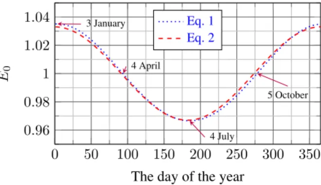
Figure 1: The calculated value of the reciprocal of the square of the Sun-Earth distance (E0) usingEqs. 1and 2
Eqs. 1and2are fromRefs.[6] and [7].E0 denotes the reciprocal of the square of the Sun-Earth distance,r0rep- resents the mean Sun-Earth distance (1 AU) andrstands for the Sun-Earth distance on the dnth day of the year.
Values ofE0using various equations are shown inFig. 1.
This change will change the solar constant too. The solar constant, I0, yields the following solar irradiance value (in W/m2) at the edge of the Earth’s atmosphere.
This constant value is1367W/m2 if the Earth is a dis- tance of 1 AU (astronomical unit) from the Sun. This value is greater at perihelion (minimum Sun-Earth dis- tance ≈ 0.983 AU on 3 January) and less at aphelion (maximum Sun-Earth distance≈ 1.017 AUon 4 July).
Since the irradiance is proportional to the surface area, which is inversely proportional to the square of the dis- tance, the corrected solar irradiance can be calculated from
In=I0E0. (3) Solar declination
The declination of the Sun,δ, yields the latitude above which the path of the Sun follows. Therefore, the zenith angle is zero at local noon. This value can be calculated from the following equations [6]:
δ= 0.006918−
−0.399912 cos
2πdn−1 365
+ + 0.070257 sin
2πdn−1 365
−
−0.006758 cos
4πdn−1 365
+ + 0.000907 sin
4πdn−1 365
−
−0.002697 cos
6πdn−1 365
+ + 0.00148 sin
6πdn−1 365
! 180°
π (4)
0 50 100 150 200 250 300 350
−23.5°
−10°
0°
10°
23.5°
20/21 March
21/22 June 22/23 September
21/22 December
The day of the year
δ Eq. 4
Eq. 5 Eq. 6 Eq. 7
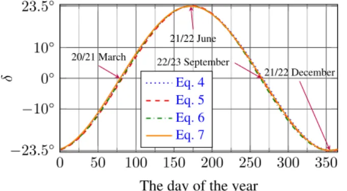
Figure 2:The calculated value of the declination of the Sun (δ) usingEqs. 4–7
δ= arcsin 0.4 sin 360
365(dn−82) !
(5) δ= 23.45°sin
2π
365(dn+ 284)
(6) and
δ= arcsin
0.39779 sin
4.8888 + 0.017214dn+ + 0.033 sin(0.017214dn)
(7) The results of different equations that calculate the dec- lination of the Sun are shown in Fig. 2. The Sun is above the equator on 20/21 March (vernal equinox) and 22/23 September (autumnal equinox), moreover, the win- ter solstice is on 21/22 December and the summer sol- stice on 21/22 June. The difference between the equa- tions inFig. 2is minimal. The maximum change in the declination when calculated on a daily basis is less than 0.5°(|δ(dn+1)−δ(dn)|).
Equation of time
A solar day varies in length throughout the year. A day on Earth is 24 hours long and is based on the rotation of the Earth around its polar axis. A solar day is based on the rotation of the Earth around its polar axis and on its mo- tion around the Sun. The elliptic orbit of the Earth causes a difference between the time of day and the solar time of day (astronomical). This means that noon in local and as- tronomical times (the Sun is in the southern hemisphere) differ.
This time difference can be calculated from the fol- lowing equations [6]:
Et=
0.000075 + 0.001868 cos
2πdn−1 365
−
−0.032077 sin
2πdn−1 365
−
−0.014615 cos
4πdn−1 365
−
−0.04089 sin
4πdn−1 365
229.18 (8)
0 50 100 150 200 250 300 350
−20
−10 0 10 20
The day of the year Et[min]
Eq. 8 Eq. 9
Eq. 10 data series†
Figure 3:The values of the Equation of Time over a year usingEqs. 8–10and a series for the year 2018
Et=h
0.043 sin
2 4.8888 + 0.017214dn+ + 0.033 sin(0.017214dn)
−
−0.03342 sin(0.017214dn)+
+ 0.2618tUTC−πi
229.18 (9)
and
Et=−7.655 sin
2πdn
365
+ + 9.873 sin
4πdn
365+ 3.588
. (10)
Eqs. 8and9yieldEtin radians and the constant229.18 converts this into minutes. This constant can be calcu- lated from
229.18 =360°
2π
360°
24·60 min16 min (11) Fig. 3shows the results according to Eqs. 8–10 over a whole year, together with astronomical data for the year 2018.
The largest difference was calculated byEq. 10when compared with the other data.
3.2 Solar beam equations
Using the equations inSection 3.1, the position and an- gles of the Sun at a local (geological) position can be cal- culated with the GPS coordinatesφlatandφlong.
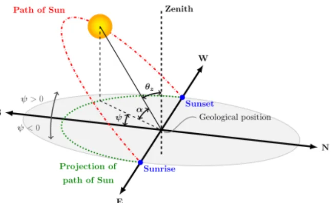
Fig. 4 shows the path of the Sun and the angles of the actual position of the Sun. The nomenclature is as follows:
• α: solar altitude angle
• θz: solar zenith angle
• ψ: solar azimuth angle
Since the altitude (α) and zenith angles (θz) are comple- mentary angles,
α+θz= 90°, (12)
the local solar hour angle can be calculated from [6]
†http://www.ppowers.com/EoT.htm
S
N
E
W Zenith
Sunset
Sunrise α ψ
θz
ψ<0 ψ>0
Geological position Path of Sun
path of Sun Projection of
Figure 4:The local position of the Sun with important angles
h= 180°−15°
tUTC+Et
60
−φlong, (13) wheretUTC is the local time in time zone+0in hours andφlongis the local longitudinal position in degrees.
The cosine of the solar zenith angle can be calculated by using the solar declination, local latitudinal position and solar hour angle. According toEq. 12,
cos(θz) = sin(δ) sin(φlat)+
+ cos(δ) cos(φlat) cos(h), (14) and
cos(θz) = sin(α), (15) (Eq. 14is fromRef.[6]) the solar azimuth angle (ψ) can be calculated from
cos(ψ) =sin(α) sin(φlat)−sin(δ)
cos(α) cos(φlat) (16) and
sin(ψ) =cos(δ) sin(h)
cos(α) . (17)
3.3 Global solar irradiance
The solar irradiance can be calculated in a simple form:
I=InqTmzsin(α), (18) whereq denotes the clear sky transmissivity through a thickness of one atmosphere,Tmrepresents the Linke tur- bidity factor of the air andzstands for the relative path length of the solar beam through the atmosphere. Parame- terqis a constant with a value of0.93(when the sky is dry and clear and the zenith angle is equal to zero). The value ofTmdetermines how many clear atmospheres should be stacked to achieve the actual spectral transmittance. This value depends on the amount of water vapor, dust, smog, etc. In the EU,Tmis between 1.8 and 4. The suggested formula for the calculation of parameterzis
z= latm
REarth−rEarth
, (19)
where latm denotes the path length of the solar beam through the atmosphere, rEarth represents the mean ra- dius of the Earth’s surface and REarth stands for the radius of the Earth when the atmosphere is included (REarth−rEarthis the thickness of the atmosphere). The value of latm depends on the solar altitude and can be calculated using the law of cosines which yields
latm2 −2rEarthlatmcos(α+ 90°)+
+ (r2Earth−R2Earth) = 0. (20) The correct value oflatmis the positive root ofEq. 20.
Eq. 18 yields the solar irradiance under ideal condi- tions. However, aerosols in the atmosphere cause diffuse scattering and absorb a proportion of the solar irradiance.
Furthermore, clouds also have an effect on the irradiance.
Some models divide the global solar irradiance into two parts:
• Direct solar irradiance
• Diffuse solar irradiance Irradiance on a horizontal surface
Various models exist to calculate the global solar irradi- ance on a horizontal surface, e.g., a Hungarian model [8]
is presented in G=
Insin(α) +a
1 +b1Nb2
, (21) where In denotes the corrected solar constant, N rep- resents the cloudy parameter between0 and1 (0 when clear, 1when overcast).ais a local correction value (a negative constant in W/m2, andb1 as well asb2are lo- cally constant in terms of the cloud correction.
This Hungarian model [8] takes the cloud cover into consideration but not the transparency of the atmosphere (q,Tmandlatm). A German model [9] accounts for at- mospheric conditions. Equation
G=Insin(α)Ade−BdTmz(1−adNbd) (22) shows the global solar irradiance and equation
S=Insin(α)AdqTmz(1−Nbd) (23) presents the direct solar irradiance formula. The param- eters ad,bd, Ad andBd are place-dependent values. A typical parameter set isad = 0.72,bd = 3.2,Ad = 0.7 andBd = 0.027. The diffuse solar irradiance can be cal- culated by a simple subtraction.
D=G−S (24)
The calculated global solar irradiance is shown in Fig.
5 over a year with weekly resolutions during clear sky conditions in Veszprém, Hungary. The red curve tracks the maximum values of the astronomical noons on each curve (analemma curve). This curve shows the effect of
5 10 15 20 0
200 400 600 800
Hour G[W/m2 ]
Global irradinace Analemma curve
Figure 5:Calculated global solar irradiance on a horizon- tal surface over the year in Veszprém according to weekly resolutions and the analemma curve (astronomical noon times)
theEt, the duration of which is approximately 11 hours because the longitudinal position of Veszprém is17.9°
and this causes a delay of about 1 hour (the local time zone is +1).
Fig. 5clearly illustrates the difference in irradiance between the winter and summer periods.
Irradiance on the slope
For the sake of simplicity the Cartesian coordinate sys- tem is used, the axes of which are S (South), W (West) and Z (Zenith). The azimuth angleψin the direction S- W-N-E-S and the altitude of the Sunαhave been calcu- lated, so the normed vector that points towards the Sun is−→
OS = [cos(α) cos(ψ), cos(α) sin(ψ), sin(α)]>. If the surface Σ exhibits an angle of inclination of β to the horizon and an orientation ofγ, which definesγas negative, positive or zero if and only if the surface faces SE, SW or S, respectively, then the normed vector of the surface (contained within the same half-space as the Sun) is−→n and exhibits the altitude ν = 90o −β so
−
→n = [cos(ν) cos(γ), cos(ν) sin(γ), sin(ν)]>. The an- gle between−→
OSand−→n is θsurf= arccos
cos(α) cos(ψ) cos(ν) cos(γ)+
+ cos(α) sin(ψ) cos(ν) sin(γ)+
+ sin(α) sin(ν)
= arccos
cos(α) cos(ν)
cos(ψ) cos(γ)+
+ sin(ψ) sin(γ)
+ sin(α) sin(ν)
, (25) since−→
OSand−→n are normed. So−→
OSmeetsΣat the angle αsurf = 90o−θsurf.
Eq. 23yields the direct solar irradiance on a horizon- tal surface with solar altitude angleα. The solar altitude
S
N
E
W Zenith
α ψ
γ O β
P Q
Surface θsurf
Figure 6:The angle of the solar beam and the zenith angle between the surface and the slopeβand orientationγ
angle on the slope isαsurf. To calculate the corrected di- rect solar irradiance, equation
Ssurf=S sin(αsurf)
sin(α) (26)
must be used. Calculation of the diffuse solar irradiance is far from trivial. If the diffuse solar irradiance is consistent with the all-sky, equation
Dsurf =D 1 + cos(β)
2 (27)
can be used to estimate the value of the irradiance. The global solar irradiance of the slope is the sum of the direct and diffuse solar irradiances:
Gsurf=Ssurf+Dsurf. (28)
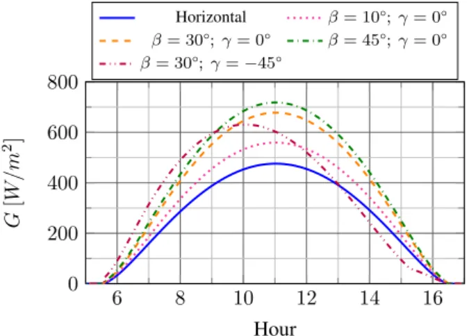
4. Model verification
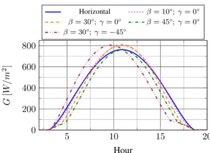
The aim of this section is to verify the solar irradiance model proposed in the previous section against basic en- gineering expectations.Figs. 7and8show the results of the implemented model on 1 March (dn= 60) and 1 July (dn = 121) and the geographical position of Veszprém, Hungary. Both figures present the value of the solar ir- radiance for various orientations as well as the tilt and azimuth angles.
6 8 10 12 14 16
0 200 400 600 800
Hour G[W/m2]
Horizontal β= 10°;γ= 0°
β= 30°;γ= 0° β= 45°;γ= 0°
β= 30°;γ=−45°
Figure 7:Calculated global solar irradiance on sloping ter- rain of various orientations on 1 March in Veszprém, Hun- gary
5 10 15 20 0
200 400 600 800
Hour G[W/m2]
Horizontal β= 10°;γ= 0°
β= 30°;γ= 0° β= 45°;γ= 0°
β= 30°;γ=−45°
Figure 8:Calculated global solar irradiance on sloping ter- rain of various orientations on 1 July in Veszprém, Hun- gary
Irradiance on a horizontal surface is denoted by a blue solid line. The other curves show the value of the solar power with a non-zero tilt angle:10° (magenta dotted line),30° (orangedashed line with an azimuth angle of zero,purpledashed dotted line with an azimuth angle of
−45° (South-East)) and45° (greendashed dotted line).
The peak values of the curves inFig. 7correlate with the tilt angle (β). As the tilt angle increases, so does the irradiance when the azimuth angle is constant (γ = 0°).
As the azimuth angle changes towards the southeast, the peak of the curve shifts towards the sunrise.
The effect of the tilt angle is somewhat different in Fig. 8. On 1 July, the absolute peak can be observed for casesβ = 10° andβ = 30° but the irradiance for the whole day is higher if the tilt angle is smaller. This ef- fect is caused by the angle of the solar altitude (smaller zenith angle). If the tilt angle is greater than the minimum horizontal zenith angle, the solar irradiance will decrease on the slope. On 1 March the maximum angle of the so- lar altitude did not reach45°. In other words, a greater tilt angle generates more power on sloping terrain. The effect of the azimuth angle can be seen inFig. 7.
5. Conclusions
A solar irradiance model is presented in this work that can be used for forecasting the solar energy absorbed by an inclined surface, e.g. a PVPP. The developed model is preliminary in nature and serves as a basis for further de- velopments, e.g. forecasting the power of the solar energy under cloudy conditions. The novel element of the model is that the relative path length of the solar beam in the atmosphere can be calculated more accurately. The cal- culated irradiance an inclined surface is exposed to is an- other novel element. The proposed model has been veri- fied against engineering expectations and the results show that it works well.
The next step will be the validation of the model us- ing real measured parameters and meteorological data.
By extending the model with an electrical power module, it will also be possible to forecast the amount of electrical energy produced.
Acknowledgement
We acknowledge the financial support of Széchenyi 2020 under the EFOP-3.6.1-16-2016-00015. We acknowledge the financial support of Széchenyi 2020 under the GINOP-2.2.1-15-2017-00038. A. Magyar was supported by the János Bolyai Research Scholarship of the Hungar- ian Academy of Sciences.
REFERENCES
[1] Braun, J.E.; Mitchell, J.C.: Solar geometry for fixed and tracking surfaces,Sol. Energy, 198331(5), 439–
444,DOI: 10.1016/0038-092X(83)90046-4
[2] Bird, R.E.; Riordan, C.: Simple solar spectral model for direct and diffuse irradiance on hor- izontal and tilted planes at the earth’s sur- face for cloudless atmospheres, J. Clim. Appl.
Meteorol., 1986 25(1), 87–97, DOI: 10.1175/1520- 0450(1986)025%3C0087:SSSMFD%3E2.0.CO;2
[3] Danandeh, M.A.; Mousavi G., S.M.: Solar irradi- ance estimation models and optimum tilt angle ap- proaches: A comparative study,Renew. Sust. Energy Rev., 201892, 319–330,DOI: 10.1016/j.rser.2018.05.004
[4] Li, D.H.W.; Chau, T.C.; Wan, K.K.W.: A review of the CIE general sky classification approaches, Renew. Sust. Energy Rev., 2014 31, 563–574, DOI:
10.1016/j.rser.2013.12.018
[5] Akarslan, E.; Hocaoglu, F.O.; Edizkan, R.:
Novel short term solar irradiance forecasting models, Renew. Energy, 2018 123, 58–66, DOI:
10.1016/j.renene.2018.02.048
[6] Iqbal, M.: An introduction to solar radiation (Academic Press, London, UK), 1st edn., 1983,
DOI: 10.1016/B978-0-12-373750-2.X5001-0, ISBN: 978-0-12- 373750-2
[7] Duffie, J.A.; Beckman, W.A.: Solar engineering of thermal processes (John Wiley & Sons, New Jersey, USA), 2013,DOI: 10.1002/9781118671603 ISBN:978-0-47- 087366-3
[8] Práger, T.; Ács, F.; Baranka, G.; Feketéné Nárai, K.; Mészáros, R.; Szepesi, D.; Weidinger, T.: A légszennyezõ anyagok transzmissziós szabványainak korszer˜usítése III. fázis Részjelentés 2., 1999 [9] Kasten, F.: Strahlungsaustausch zwischen Ober-
flächen und Atmosphäre, VDI-Bericht, 1989 (Nr.
721. S.), 131–158
Appendix: Nomenclature
Symbol Description Value/dimension
E0 Reciprocal of the relative Sun-Earth squared distance (r0/r)2 r0 Mean Sun-Earth distance (Astronomical Unit: [AU]) 1 AU
r Actual Sun-Earth distance inAU [AU]
dn The day of the year 1-365
I0 Solar constant 1367W/m2
In Corrected solar constant I0E0
δ Sun’s declination ±23.5°
Et Equation of time ∼ ±15 min
tUTC The time in UTC 0-24
φlat Geographic latitude ±90°
φlong Geographic longitude ±180°
α The angle of the solar altitude 0°-90°
θz Solar zenith angle 90°−α
ψ Solar azimuth angle ±180°
h The solar hour angle 0°-360°
q Clear sky transmissivity 0.93
Tm Linke turbidity factor 1.8-4 in Central EU
z Relative solar beam length in the atmosphere
latm Length of the path of the solar beam through the atmosphere [km]
REarth Median radius of the Earth including the atmosphere ∼6470km rEarth Median radius of the Earth from the ground ∼6370km
G Global solar irradiance [W/m2]
N Cloudy parameter 0-1
Ad Place-dependent constant
Bd Place-dependent constant
ad Place-dependent constant
bd Place-dependent constant
D Diffuse solar irradiance [W/m2]
S Direct solar irradiance [W/m2]
β Angle above the surface from the horizontal position 0°–90°
γ Surface azimuth angle ±90°
θsurf The solar zenith angle on the surface 90°−αsurf
αsurf The angle of the solar altitude on the surface 0°-90°
Ssurf Direct solar irradiance on the surface [W/m2]
Dsurf Diffuse solar irradiance on the surface [W/m2]
Gsurf Global solar irradiance on the surface [W/m2]