ANNALES
MATHEMATICAE ET INFORMATICAE
VOLUME 36. (2009)
EDITORIAL BOARD
Sándor Bácsó (Debrecen), Sonja Gorjanc (Zagreb), Tibor Gyimóthy (Szeged), Miklós Hoffmann (Eger), József Holovács (Eger), László Kozma (Budapest), Kálmán Liptai (Eger), Florian Luca (Mexico), Giuseppe Mastroianni (Potenza), Ferenc Mátyás (Eger), Ákos Pintér (Debrecen), Miklós Rontó (Miskolc, Eger), László Szalay (Sopron), János Sztrik (Debrecen, Eger), Gary Walsh (Ottawa)
INSTITUTE OF MATHEMATICS AND INFORMATICS ESZTERHÁZY KÁROLY COLLEGE
HUNGARY, EGER
HU ISSN 1787-5021 (Print) HU ISSN 1787-6117 (Online)
A kiadásért felelős:
az Eszterházy Károly Főiskola rektora Megjelent az EKF Líceum Kiadó gondozásában
Kiadóvezető: Kis-Tóth Lajos Felelős szerkesztő: Zimányi Árpád Műszaki szerkesztő: Tómács Tibor Megjelent: 2009. december Példányszám: 50
Készítette:
az Eszterházy Károly Főiskola nyomdája Felelős vezető: Kérészy László
Annales Mathematicae et Informaticae 36(2009) pp. 3–14
http://ami.ektf.hu
A common fixed point theorem via a generalized contractive condition
Abdelkrim Aliouche
a, Faycel Merghadi
baDepartment of Mathematics, University of Larbi Ben M’Hidi Oum-El-Bouaghi, Algeria
bDepartment of Mathematics, University of Tebessa, Algeria Submitted 8 January 2009; Accepted 12 June 2009
Abstract
We prove a common fixed point theorem for mappings satisfying a gener- alized contractive condition which generalizes the results of [3, 4, 12, 15, 19, 20, 24] and we correct the errors of [7, 12, 20].
Keywords: Metric space, weakly compatible mappings, common fixed point.
MSC:47H10, 54H25
1. Introduction
Sessa [21] defined S and T to be weakly commuting as a generalization of commuting if for allx∈X.
d(ST x, T Sx)6d(T x, Sx).
Jungck [9] defined S and T to be compatible as a generalization of weakly com- muting if
n→∞lim d(ST xn, T Sxn) = 0
whenever{xn} is a sequence in X such thatlimn→∞Sxn = limn→∞T xn =t for somet∈X. It is easy to show that commuting implies weakly commuting implies compatible and there are examples in the literature verifying that the inclusions are proper, see [9, 21]. Jungck et al [10] definedS andT to be compatible mappings of type (A) if
n→∞lim d ST xn, T2xn
= 0 and lim
n→∞d T Sxn, S2xn
= 0,
3
4 A. Aliouche, F. Merghadi whenever{xn} is a sequence in X such thatlimn→∞Sxn = limn→∞T xn =t for some t ∈ X. Example are given to show that the two concepts of compatibility are independent, see [10]. Recently, Pathak and Khan [16] definedS andT to be compatible mappings of type (B) as a generalization of compatible mappings of type (A) if
n→∞lim d T Sxn, S2xn 61
2 h
n→∞lim d(T Sxn, T t) + lim
n→∞d T t, T2xni ,
n→∞lim d ST xn, T2xn 61
2 h
n→∞lim d(ST xn, St) + lim
n→∞d St, S2xni ,
whenever{xn} is a sequence in X such thatlimn→∞Sxn = limn→∞T xn =t for somet∈X. Clearly compatible mappings of type (A) are compatible mappings of type (B), but the converse is not true, see [16]. However, compatible mappings of type (A) and compatibility of type (B) are equivalent if S andT are continuous, see [16]. Pathak et al [17] definedS andT to be compatible mappings of type (P) if
n→∞lim d S2xn, T2xn
= 0,
whenever{xn} is a sequence in X such thatlimn→∞Sxn = limn→∞T xn =t for somet∈X. However, compatibility, compatibility of type (A) and compatibility of type (P) are equivalent if S and T are continuous, see [17]. Pathak et al [18]
defined S and T to be compatible mappings of type (C) as a generalization of compatible mappings of type (A) if
nlim→∞
d T Sxn, S2xn
6 1 3 h
nlim→∞
d(T Sxn, T t) + lim
n→∞
d T t, S2xn
+ lim
n→∞
d T t, T2xn
i,
nlim→∞
d ST xn, T2xn
6 1 3 h
nlim→∞
d(ST xn, St) + lim
n→∞
d St, T2xn
+ lim
n→∞
d St, S2xn
i, whenever{xn} is a sequence in X such thatlimn→∞Sxn = limn→∞T xn =t for some t ∈ X. Compatibility, compatibility of type (A) and compatibility of type (C) are equivalent if S andT are continuous, see [18]. Pant [15] definedS andT to be reciprocally continuous if
n→∞lim ST xn=Stand lim
n→∞T Sxn=T t,
whenever {xn} is a sequence in X such that limn→∞Sxn = limn→∞T xn = t for some t ∈ X. It is clear that if S and T are both continuous, then they are reciprocally continuous, but the converse is not true. Moreover, it was proved in [15] that in the setting of common fixed point theorem for compatible mappings satisfying contractive conditions, the continuity of one of the mappings S and T implies their reciprocal continuity, but not conversely.
2. Preliminaries
Definition 2.1 (See [11]). S andT are said to be weakly compatible if they com- mute at their coincidence points; i.e., ifSu=T ufor someu∈X, thenST u=T Su.
A common fixed point theorem via a generalized contractive condition 5 Lemma 2.2 (See [9, 10, 16, 17, 18]). If S andT are compatible, or compatible of type (A), or compatible of type (P), or compatible of type (B), or compatible of type (C), then they are weakly compatible.
The converse is not true in general, see [4].
Definition 2.3 (See [13]). S andT are said to be R−weakly commuting if there exists anR >0such that
d(ST x, T Sx)6Rd(T x, Sx) for allx∈X. (2.1) Definition 2.4 (See [14]). S and T are pointwiseR−weakly commuting if for all x∈X, there exists anR >0 such that (2.1) holds.
It was proved in [14] that R-weakly commutativity is equivalent to commuta- tivity at coincidence points; i.e.,SandT are pointwiseR-weakly commuting if and only if they are weakly compatible.
Lemma 2.5 (See [22]). For any t∈(0,∞),ψ(t)< t ifflimn→∞ψn(t) = 0, where ψn denotes the n-times repeated composition ofψwith itself.
Several authors proved fixed point and common fixed point theorem for map- pings satisfying contractive conditions of integral type, see [1, 3, 4, 5, 6, 7, 12, 19, 20]. The following theorem was proved by [3].
Theorem 2.6 (See [3]). Let A, B, S and T be self-mappings of a metric space (X, d)satisfying
S(X)⊂B(X) and T(X)⊂A(X), Z d(Sx,T y)
0
ϕ(t) dt6ψ
Z M(x,y) 0
ϕ(t) dt
!
for all x, y ∈ X, ψ:R+ →R+ is a right continuous function such that ψ(0) = 0 andψ(s)< sfor alls >0andϕ: R+→R+is a Lebesgue integrable mapping which is summable and satisfies Z ǫ
0
ϕ(t) dt >0, M(x, y) = max
d(Ax, By), d(Sx, Ax), d(T y, By),1
2[d(Sx, By) +d(T y, Ax)]
. If one of A(X), B(X), S(X)andT(X)is a complete subspace ofX, thenAand S have a coincidence point and B andT have a coincidence point. Further, if S andAas well asT andB are weakly compatible, thenA, B, S andT have a unique common fixed point inX.
Recently, Zhang [24] and Aliouche [2] proved common fixed point theorems using generalized contractive conditions in metric spaces.
LetA∈(0,∞],RA+= [0, A)andF:RA+→Rsatisfying
6 A. Aliouche, F. Merghadi (i)F(0) = 0andF(t)>0 for eacht∈(0, A),
(ii)F is nondecreasing onR+A, (iii)F is continuous.
Define̥[0, A) ={F :F satisfies (i)–(iii)}.
Lemma 2.7 (See [24]). Let A ∈ (0,∞], F ∈ ̥[0, A). If limn→∞F(ǫn) = 0 for ǫn ∈R+A, thenlimn→∞ǫn= 0.
The following examples were given in [24].
(i) LetF(t) =t, thenF ∈̥[0, A)for eachA∈(0,∞].
(ii) Suppose thatϕis nonnegative, Lebesgue integrable on[0, A)and satisfies Z ǫ
0
ϕ(t) dt >0for eachǫ∈(0, A).
LetF(t) =Rt
0ϕ(s) ds, thenF ∈[0, A).
(iii) Suppose thatψis nonnegative, Lebesgue integrable on[0, A)and satisfies Z ǫ
0
ψ(t) dt >0 for eachǫ∈(0, A) andϕis nonnegative, Lebesgue integrable onh
0,RA
0 ψ(s) ds
and satisfies Z ǫ
0
ϕ(t) dt >0 for each0< ǫ <
Z A 0
ψ(s) ds.
LetF(t) =RR0tψ(s) ds
0 ϕ(u) du, thenF ∈̥[0, A).
(iv) If G ∈ [0, A) and F ∈ ̥[0, G(A −0)), then a composition mapping F ◦G∈̥[0, A). For instance, letH(t) =RF(t)
0 ϕ(s) ds, then H ∈ ̥[0, A)when- everF ∈̥[0, A)andϕis nonnegative, Lebesgue integrable on̥[0, F(A−0))and
satisfies Z ǫ
0
ϕ(t) dt >0 for eachǫ∈(0, F(A−0)).
LetA∈(0,∞]andψ:R+A →R+ satisfying (i)ψ(t)< tfor allt∈(0, A)
(ii)ψis upper semi-continuous.
(iii)ψis nondecreasing onR+A,
DefineΨ[0, A) ={ψ:ψsatisfies (i)-(iii)}.
3. Main results
Theorem 3.1. Let (X, d)be a metric space and D= sup{d(x, y) :x, y∈X}. Set A=D if D=∞ andA > D ifD <∞. LetA1, A2, S andT be self-mappings of (X, d)satisfying
A1(X)⊂T(X)andA2(X)⊂S(X),
A common fixed point theorem via a generalized contractive condition 7 F(d(A1x, A2y))6ψ(F(L(x, y))) (3.1) for all x, y inX, where
L(x, y) = maxn
d(Sx, T y), d(A1x, Sx), d(T y, A2y),1
2[d(Sx, A2y) +d(A1x, T y)]o , F ∈ ̥[0, A) and ψ ∈ Ψ[0, F(A−0)) for all A ∈ (0,∞]. Suppose that the pair (A1, S)is weakly compatible and there exists w∈C(A2, T): the set of coincidence points ofA2andT such thatA2T w=T A2w. If one ofA1(X), A2(X), S(X)and T(X) is a complete subspace ofX, then A1, A2, S and T have a unique common fixed point in X.
Proof. Letx0be arbitrary point inX. Inductively, we can define a sequence{yn} in X such that
y2n =A1x2n=T x2n+1andy2n+1=Sx2n+2=A2x2n+1
for all n = 0,1,2, . . .. As in the proof of [2], {yn} is a Cauchy sequence in X. Assume thatS(X)is complete. Therefore
n→∞lim A1x2n= lim
n→∞T x2n+1= lim
n→∞A2x2n+1= lim
n→∞Sx2n+1=z=Su for some u∈X. IfA1u6=z using (3.1) we obtain
F(d(A1u, A2x2n+1))6ψ(F(L(u, x2n))) where
L(u, x2n) = maxn
d(Su, T x2n+1), d(A1u, Su), d(T x2n+1, A2x2n+1), 1
2[d(Su, A2x2n+1) +d(A1u, T x2n+1)]o . Letting n→ ∞, we get
F(d(A1u, z))6ψ(F(d(A1u, z)))< F(d(A1u, z))
which is a contradiction and so z = A1u = Su. Ifz 6= A2w, applying (3.1) we obtain
F(d(A1u, A2w))6ψ(F(d(A1u, A2w))) where
L(u, v) = maxn
d(Su, T w), d(A1u, Su), d(T w, A2w),1
2[d(Su, A2w) +d(A1u, T w)]o . Hence
F(d(z, A2w))6ψ(F(d(z, A2w)))< F(d(z, A2w)).
which is a contradiction and so z=A1u=Su=A2w=T w.
8 A. Aliouche, F. Merghadi Since the pairs(A1, S)is weakly compatible and there existsw∈C(A2, T)such that A2T w=T A2w, we haveSz=A1z andT z=A2z.
IfA1z6=z we have by (3.1)
F(d(A1z, A2w))6ψ(F(L(z, w))) where
L(z, w) = maxn
d(Sz, T w), d(A1z, Sz), d(Bw, A2w),1
2[d(Sz, A2w) +d(A1z, T w)]o . Therefore
F(d(A1z, z))6ψ(F(d(A1z, z)))< F(d(A1z, z)) and so A1z=Sz=z. Similarly, we can prove thatA2z=T z=z.
The proof is similar when T(X)is assumed to be a complete subspace of X.
The case in whichA1(X)orA2(X)is a complete subspace ofX is similar to the case in which T(X)or S(X) respectively is complete since A1(X)⊂T(X)and A2(X)⊂S(X). The uniqueness ofz follows from (3.1).
Theorem 3.1 generalizes Theorem 2.6 of [3].
Corollary 3.2. Let (X, d) be a metric space and D = sup{d(x, y) : x, y ∈ X}. Set A =D if D =∞ andA > D if D <∞. Let {Ai},i = 1,2, . . . , S andT be self-mappings of (X, d)satisfying
A1(X)⊂T(X)andAi(X)⊂S(X),i>2 and
F(d(A1x, Aiy))6ψ(F(Li(x, y))),i>2 for all x, y inX, where
Li(x, y) = maxn
d(Sx, T y), d(A1x, Sx), d(Aiy, T y),1
2[d(Sx, Aiy) +d(A1x, T y)]o , F ∈ ̥[0, A) and ψ ∈ Ψ[0, F(A−0)) for all A ∈ (0,∞]. Suppose that the pair (A1, S)is weakly compatible and there existsw∈C(Ai, T): the set of coincidence points ofAi andT such thatAiT w=T Aiwfor somei>2. If one ofAi(X), S(X) andT(X)is a complete subspace ofX. ThenAi, S andT have a unique common fixed point in X.
Ifϕ(t) = 1in Corollary 3.2, we get a generalization of a theorem of [15]. The following example illustrates our corollary 3.2.
Example 3.3. LetX = [0,10]be endowed with the metricd(x, y) =|x−y|,
Sx=
0, ifx= 0, x+ 8, ifx∈(0,2], x−2, ifx∈(2,10],
T x=
0, ifx= 0, x+ 5, ifx∈(0,2], x−2, ifx∈(2,10],
A common fixed point theorem via a generalized contractive condition 9
A1x=
(3, ifx∈(0,2],
0, ifx∈ {0} ∪(2,10], A2x=
(0, ifx∈[0,2], 4, ifx∈(2,10], A3x=
(0, ifx∈[0,2],
5, ifx∈(2,10], A4x=
(0, ifx∈[0,2], 6, ifx∈(2,10], Aix=
(2 + 2i, ifx∈(0,2],
0, ifx∈ {0} ∪(2,10], for alli >4.
The pair (A1, S) is weakly compatible, but it is not compatible of type (A), (B), (P) and (C), see [6].
A1(X)⊂T(X)andAi(X)⊂S(X).
The pair(Ai, T), i >4, is weakly compatible becauseAi and T commute at their coincidence point x= 0, but it is not compatible of type (A), (B), (P) and (C).
Letxn= 2 + 1n. We haveT xn= n1 andAixn= 0,hence
n→∞lim T xn= lim
n→∞Aixn =t= 0.
In the other hand, AiT xn = Ai(n1) = 2 + 2i and T Aixn = T0 = 0 and so limn→∞d(AiT xn, T Aixn) = 2 +2i 6= 0.Therefore, the pair(Ai, T)is not compat- ible.
A2ixn =Ai0 = 0and T2xn=T n1
= 5 +n1, so limn→∞
T Aixn−A2ixn
= 0 andlimn→∞
AiT xn−T2xn
= limn→∞(3 +n1−2i)6= 0for alli >3. Then,(Ai, T) is not compatible of type (A).
n→∞lim
AiT xn−T2xn
= 3−2 i > 1
2 h
n→∞lim |AiT xn−Ai0|+ lim
n→∞
Ai0 −A2ixn
i
=1 2 2 +2
i =1
i + 1, hence (Ai, T)is not compatible of type (B).
limn→∞
A2ixn−T2xn
= limn→∞(5 + n1) = 5 6= 0. Therefore, (Ai, T)is not compatible of type (P).
n→∞lim
AiT xn−T2xn
= 3−2 i
> 1 3
h lim
n→∞|AiT xn−Ai0|+ lim
n→∞
Ai0−T2xn
+ lim
n→∞
Ai0 −A2ixn
i
= 1 3
7 + 2
i
fori >4. So, the pair(Ai, T)is not compatible of type (C).
It can be verified that the pairs (A2, T) , (A3, T) and (A4, T)are not weakly compatible because x = 6 is a coincidence point ofA2 and T, butA2T6 = 4 6=
10 A. Aliouche, F. Merghadi T A26 = 2,x= 7is a coincidence point ofA3andT, butA3T(7) = 56=T A3(7) = 3 andx= 8is a point of coincidence forA4andT, but A4T(8) = 66=T A4(8) = 4.
Now, we begin to verify the rest of conditions of Corollary 3.2. Let F(t) = ln(1 +t)andψ(t) =ht, where06h <1and t >0. Set
R= ln(1 +|A1x−Aiy|)−hmax
ln(1 +|Sx−T y|),ln(1 +|A1x−Sx|), ln(1 +|Aiy−T y|),
1
2[ln(1 +|A1x−T y|) + ln(1 +|Sx−Aiy|)]
We have the following cases. Ifx= 0andy= 0we getR60for all06h <1.If x= 0andy∈(0,2], we get
R= ln
3 +2 i
−hmax
ln (y+ 6),ln y+ 4−2i
,
1 2
ln (y+ 6) + ln 3 +2i
60 forh>ln(3+2i)
3 ln 2 and so there exists06h <1.Ifx= 0andy∈(2,10],we get R=−hmax{ln (y−1),ln (y−1),ln (y−1)}60
for all06h <1. Ifx∈(0,2]andy= 0, we get R= ln 4−hmax
ln (x+ 9),ln (x+ 6),
1
2[ln 4 + ln (x+ 9)]
60 forh> ln 4
ln 11 and so there exists06h <1. Ifx∈(0,2]andy∈(0,2],we get R= ln
2−2
i
−hmax
ln(x−y+ 4),ln(x+ 6),ln y+ 4−2i
,
1 2
ln (y+ 3) + ln x+ 7−2i
60 forh>ln(3−2i)
ln 8 .Hence, there exists06h <1.Ifx∈(0,2]andy∈(2,10],we get R= ln 4−hmax
ln (x+ 11−y),ln (x+ 6),ln (y−1),
1
2[ln (|5−y|+ 1) + ln (x+ 9)]
60 forh>ln 11ln 4.Hence, there exists06h <1.Ifx∈(2,10]andy= 0, we get
R=−hmax
ln (x−1),ln (x−1),0,1
2ln (x−1)
60
for allh>0.Hence, there exists06h <1.Ifx∈(2,10]andy∈(0,2],we get R= ln
3 +2
i
−hmax
ln (|x−(y+ 7)|+ 1),ln (x−1), ln y+ 3−2i
,12
ln (y+ 5) + ln x−4−2i
+ 1
60 forh>ln(3+2i)
ln 9 .Hence, there exists06h <1.Ifx, y∈(2,10]we get R=−hmax
ln (|x−y|+ 1),ln (x−1),ln (y−1),
1
2[ln (y−1) + ln (x−1)]
60
A common fixed point theorem via a generalized contractive condition 11 for all06h <1.
Now, we verify that (A2, T) and (A3, T) satisfy all the conditions of Theo- rem 4.2. Set
R1=
Z |A1x−A2y|
0
1 1 +tdt−
−hmax
R|Sx−T y|
0
1
1+tdt,R|A1x−Sx|
0
1
1+tdt,R|A2y−T y|
0
1 1+tdt,
1 2
hR|A1x−T y|
0
1
1+tdt+R|Sx−A2y|
0
1 1+tdti
We have the following cases. If x= 0and y= 0we get R160for all 06h <1.
Ifx= 0andy∈(0,2], we get R1=−hmax
ln (y+ 6),0,ln (y+ 6),1 2[y+ 6]
60 for all06h <1.Ifx= 0andy∈(2,10],we get
R1= ln 5−hmax
ln (y−1),ln (|y−6|+ 1),
1
2[ln (y−1) + ln 5]
60 forh>ln 5
ln 9,hence there exists06h <1.Ifx∈(0,2]andy= 0, we get R1= ln 4−hmax
ln (x+ 9),ln (x+ 6),0,
1
2[ln 4 + ln (x+ 9)]
60 for allh> ln 4
ln 11.Hence, there exists06h <1.Ifx∈(0,2]andy∈(0,2],we get R1= ln 4−hmax
ln (4 +x−y),ln (x+ 6),ln (y+ 6),
1
2[ln (y+ 3) + ln (x+ 9)]
60 forh>ln 4ln 8. Hence there exists06h <1.Ifx∈(0,2]andy∈(2,10],we get
R1= ln 2−hmax
ln 11,ln (x+ 6),ln (|y−6|+ 1),
1
2[ln (|5−y|+ 1) + ln (x+ 5)]
60 forh>ln 11ln 2.Hence,there exists06h <1.Ifx∈(2,10]andy= 0, we get
R1=−hmax
ln (x−1),ln (x−1),1
2ln (x−1)
60
for all06h <1. In the same manner, if x∈(2,10]andy ∈(0,2],we getR160 for all06h <1.Ifx∈(2,10]andy∈(2,10],we get
R1= ln 5−hmax
ln (|x−y|+ 1),ln (x−1),ln (|y−6|+ 1),
1
2[ln (y−1) + ln|x−6|+ 1]
60
12 A. Aliouche, F. Merghadi for h> ln 5ln 9. Hence, there exists 06h <1.Similarly, we can prove the conditions of Theorem 4.2 if we take the mapping A3 instead ofA2. Finally we remark that all conditions of our theorem are verified and 0 is the unique common fixed point ofAi, S andT.
The following example support our Theorem 3.1.
Remark 3.4. In this example, Theorem 2.6 of [3] is not applicable since the pair (A2, T)is not weakly compatible, but Theorem 3.1 is applicable. Also, a theorem of [15] forAi =A2 for alli>2is not applicable since the pairs(A1, S)and(A2, T) are not compatible. In the same manner, Theorem 1 of [12] is not applicable.
Remark 3.5. In the proof of Lemma 1 of [20] and Theorem 2.1 of [7], the authors applied the inequality
a6b+c=⇒ Z a
0
ϕ(t)dt6 Z b
0
ϕ(t)dt+ Z c
0
ϕ(t)dt which is false in general as it is shown by the following example.
Example 3.6. Letϕ(t) =t,a= 1,b= 12 andc= 34. Then1< 12+34, but Z 1
0
ϕ(t)dt=1 2 >
Z 12
0
ϕ(t)dt+ Z 34
0
ϕ(t)dt
=1 8 + 9
32 =13 32.
To correct these errors, the authors should follow the proof of Theorem 2 of [19].
Remark 3.7. In the proof of Theorem 1 of [12], the authors applied the inequality
n→∞lim d(xn, xn+1) = 0 =⇒ {xn} is a Cauchy sequence
which is false in general. It suffices to take xn =n1, n∈N∗. Thus, To correct this error, the authors should follow the proof of Theorem 2 of [19].
References
[1] Aliouche, A., A common fixed point theorem for weakly compatible mappings in symmetric spaces satisfying a contractive condition of integral type, J. Math. Anal.
Appl., 322 (2) (2006), 796–802.
[2] Aliouche, A., Common fixed point theorems of Gregus type for weakly compatible mappings satisfying generalized contractive conditions,J. Math. Anal. Appl., 341 (1) (2008), 707–719.
A common fixed point theorem via a generalized contractive condition 13 [3] Altun, I., Turkoglu, D., Rhoades, B.E., Fixed points of weakly compatible mappings satisfying a general contractive condition of integral type, Fixed Point Theory And Applications, Volume 2007 (2007), Article ID 17301, 9 pages.
[4] Branciari, A., A fixed point theorem for mappings satisfying a general contractive condition of integral type,Int. J. Math. Math. Sci., 29 (2002), 531–536.
[5] Djoudi, A., Aliouche, A., Common fixed point theorems of Gregus type for weakly compatible mappings satisfying contractive conditions of integral type, J.
Math. Anal. Appl., 329 (1) (2007), 31–45.
[6] Djoudi, A., Merghadi, F., Common fixed point theorems for maps under a con- tractive condition of integral type,J. Math. Anal. Appl., 341 (2) (2008), 953–960.
[7] Gairola, U.C., Rawat, A.S., A fixed point theorem for integral type inequality, Int. Journal of Math. Analysis, Vol. 2, 2008, no. 15, 709–712.
[8] Bouhadjera, H., Djoudi, A., Common fixed point theorems for pairs of single and multivalued D-maps satisfying an integral type, Annales Math. et Inf., 35, (2008), 43–59.
[9] Jungck, G., Compatible mappings and common fixed points,Int. J. Math. Math.
Sci., 9 (1986), 771–779.
[10] Jungck, G., Murthy, P.P., Cho, Y.J., Compatible mappings of type (A) and common fixed points,Math. Japonica., 38 (2) (1993), 381–390.
[11] Jungck, G., Common fixed points for non-continuous non-self maps on non metric spaces,Far East J. Math. Sci., 4 (2) (1996), 199–215.
[12] Kohli, J.K., Vashistha, S., Common fixed point theorems for compatible and weakly compatible mappings satisfying general contractive type conditions,Studii şi Cercetări Ştiinţifice, Seria Matematică, Universitatea din Bacău, 16 (2006), 33–42 [13] Pant, R.P., Common fixed points of noncommuting mappings,J. Math. Anal. Appl.,
188 (1994), 436–440.
[14] Pant, R.P., Common fixed points for four mappings,Bull. Calcutta. Math. Soc., 9 (1998), 281–286.
[15] Pant, R.P., A Common fixed point theorem under a new condition,Indian J. Pure.
Appl. Math., 30 (2) (1999), 147–152.
[16] Pathak, H.K., Khan, M.S., Compatible mappings of type (B) and common fixed point theorems of Gregus type,Czechoslovak Math. J., 45 (120) (1995), 685-698.
[17] Pathak, H.K., Cho, Y.J., Kang, S.M., Lee, B.S., Fixed point theorems for compatible mappings of type (P) and applications to dynamic programming, Le Matematiche, 1 (1995), 15–33.
[18] Pathak, H.K., Cho, Y.J., Khan, S.M., Madharia, B., Compatible mappings of type (C) and common fixed point theorems of Gregus type,Demonstratio Math., 31 (3) (1998), 499–518.
[19] Rhoades, B.E., Two fixed point theorems for mappings satisfying a general con- tractive condition of integral type,Int. J. Math. Math. Sci., 63 (2003), 4007–4013.
[20] Vijayaraju, P., Rhoades, B.E., Mohanraj, R., A fixed point theorem for a pair of maps satisfying a general contractive condition of integral type,Int. J. Math.
Math. Sci., 15 (2005), 2359–2364.
14 A. Aliouche, F. Merghadi [21] Sessa, S., On a weak commutativity condition of mappings in fixed point consider-
ations,Publ. Inst. Math. Beograd., 32 (46) (1982), 149–153.
[22] Singh, S.P., Meade, B.A., On common fixed point theorems,Bull. Austral. Math.
Soc., 16 (1977), 49–53.
[23] Suzuki, T., Meir-Keeler contractions of integral type are still Meir-Keeler con- tractions, Int. J. Math. Math. Sci., 2007, Article ID 39281, 6 pages, 2007.
doi:10.1155/2007/39281.
[24] Zhang, X., common fixed point theorems for some new generalized contractive type mappings,J. Math. Anal. Appl., 333 (2) (2007), 780–786.
A. Aliouche
Department of Mathematics
University of Larbi Ben M’Hidi Oum-El-Bouaghi 04000
Algeria
e-mail: alioumath@yahoo.fr F. Merghadi
Department of Mathematics University of Tebessa 12000
Algeria
e-mail: faycel_mr@yahoo.fr
Annales Mathematicae et Informaticae 36(2009) pp. 15–28
http://ami.ektf.hu
Approximation approach to performance evaluation of Proxy Cache Server systems
Tamás Bérczes
Department of Informatics Systems and Networks, University of Debrecen Submitted 8 January 2009; Accepted 15 April 2009
Abstract
In this paper we treat a modification of the performance model of Proxy Cache Servers to a more powerful case when the inter-arrival times and the service times are generally distributed. First we describe the original Proxy Cache Server model where the arrival process is a Poisson process and the service times are supposed to be exponentially distributed random variables.
Then we calculate the basic performance parameters of the modified perfor- mance model using the well known Queueing Network Analysis (QNA) ap- proximation method. The accuracy of the new model is validated by means of a simulation study over an extended range of test cases.
Keywords: Queueing Network, Proxy Cache Server, Performance Models, GI/G/1 queue
1. Introduction
The Internet quickly became an essential and integral part of today’s life. How- ever, the booming use of the Web has caused congested networks and overloaded servers. So, the answer from the remote Web server to the client often takes a long time. Adding more network bandwidth is a very expensive solution. From the user’s point of view it does not matter whether the requested files are on the firm’s computer or on the other side of the world. The main problem is that the same object can be requested by other users at the same time. Because of this situation, identical copies of many files pass through the same network links, resulting in an increased response time. By preventing future transfer, we can cache information and documents that reduces the network bandwidth demand on the external net- work. In general, there are three types of caches that can be used in isolation or in a hierarchical fashion. Caching can be implemented at browser software [2]; the originating Web sites [3]; and the boundary between the local area network and the
15
16 T. Bérczes Internet [4]. Browser cache are inefficient since they cache for only one user. Web server caches can improve performance, although the requested files must delivery through the Internet, increasing the response time. In this paper we investigate the third type. Requested documents can be delivered directly from the Web server or through a Proxy Cache Server (PCS). A PCS has the same functionality as a Web server when looked at from the client and the same functionality as a client when looked at from a Web server. The primary function of a PCS is to store documents close to the users to avoid retrieving the same document several times over the same connection. It has been suggested that, given the current state of technology, the greatest improvement in response time will come from installing a PCS at the boundary between the corporate LAN and the Internet.
In this paper, we present an extended version of the performance model of a PCS (see [5, 7]) using a more powerful case when inter-arrival times and the service times are generally distributed.
The organization of the paper is as follows. In Section 2, renewal-based para- metric decomposition models are reviewed (see [1, 10]). In Section 3 we introduce a modified version of the original performance model of Proxy Cache Server, where we include the repetition loop at the Proxy Server. A detailed description of the generalized model is given in Section 4. Section 5 is devoted to the validation of the numerical results of the approximation. The paper ends with Comments.
2. The GI/G/1 approximation
The GI/G/1 approximation described here is an example of a method using Parametric Decomposition (see [10]) where the individual queueing nodes are an- alyzed in isolation based on their respective input and output processes. In this model, the arrival process is a general (GI) arrival process characterised by a mean arrival rate and a squared coefficient of variation (SQV) of the inter-arrival time and the service time may have any general distribution. To use the approxima- tion, we need only to know the mean and the squared coefficient of variance of the inter-arrival times and the service times. In order to apply this method, we assume that the arrival process to a network node is renewal, so the arrival intervals are independent, identically distributed random variables. Immediate feedback, where a fraction of the output of a particular queue enters the queue once again, needs special treatment. Before the detailed analysis of the queueing network is done, the method first removes immediate feedback in a queue by suitably modifying its service time.
This model contains procedures required for modeling of the basic network op- erations of merging, departure and splitting, arising due to the common sharing of the resources and routing decisions in the network. Futhermore, the approximation provide performance measures (i.e. mean queue lengths, mean waiting times, etc.) for both per-queue and per-network.
The parameters required for the approximation: Arrival process: (λA - the mean arrival rate), (c2A - the SQV of the inter-arrival time) and service time (τS
Approximation approach to performance evaluation of Proxy Cache Server systems 17 - the mean service time), and (c2S - the SQV of the service time) at a considered node.
The approximation method that transforms the two parameters of the inter- nal flows for each of the three basic network operations and the removal of the immediate feedback, as given in [1], is described in the following:
1) Merging GI traffic flows: The superposed process of n individual GI flows, each characterized by λj and c2j (j = 1, . . . , n), as it enters the considered node is approximated by a GI traffic flow with parameters λA and c2S, representing the mean arrival rate and SQV of the inter-arrival time of the superposed flow, respectively. The mean arrival rate and the SQV of the inter-arrival time of the superposed flow is given by:
λA= Xn j=1
λj,
c2A=̟ Xn j=1
λj
λAc2j+ 1−̟, with
̟= 1
1 + 4(1−ρ)2(ν−1),
ν = 1
Pn j=1
λ
j
λA
2,
andρis the utilisation at the node, defined byρ=λAτS.
2) Departure flow from a queue: The departure flow from a queue is approx- imated as a GI traffic flow, characterized by λD and c2D, representing the mean departure rate and SQV of the inter-departure time of the departure flow, respec- tively. Under equilibrium conditions, the mean flow entering a queue is always equal to the mean flow existing the queue: λD=λA. The SQV of inter-departure time of the departure flow is given by:
c2D=ρ2c2S+ 1−ρ2 c2A
3)Splitting a GI flow Probabilistically: If a GI flow with parametersλandc2is split into n flows, each selected independently with probabilitypi, the parameters for the i-th flow will be given by:
λi =piλ, c2i =pic2+ (1−pi).
4)Removing immediate feedback: If the output traffic from a queue is fed back to this queue itself (Qi), so that the net arrival process is the sum of the external
18 T. Bérczes arrivalsΛand the fed back portionpiiλi. The approach followed to eliminate this immediate feedback at the queue is to suitably adjust the service time at the queue and the SQV of service time. Assume that the original service parameters at the considered node are: τS,U- the mean service time, andc2S,U - the SQV of the service time. Removing the immediate feedback from that node we will get the modified service parameters:
τS,M = τS,U
1−pii
, c2S,M =pii+ (1−pii)c2S,U,
Wq,M = Wq,M
1−pii
.
This reconfigured queue without immediate feedback is used subsequently for solv- ing the queueing network.
5)Mean waiting time: If the considered node is a GI/G/1 queue, the following Kramer and Langenbach-Belz approximation is used (see [12]):
Wq =τS·ρ(c2A+c2D)β 2(1−ρ) with
βW eb=
(exp2(1−ρ)(1−c2 A)2 3ρ(c2A+c2D)
, forc2A<1,
1 forc2A>1.
3. The model of Proxy Cache Server
In this section we modified the original (M/M/1) performance model of Proxy Cache Server (see [5]). In this version of the performance model the Proxy Cache Server behaves like a Web server. So, if the size of the file that will pass through the server, is greater then the server’s output buffer it will start a looping process until the delivery of all file’s is completed (see [11, 6]).
Using Proxy Cache Server, if any information or file is requested to be down- loaded, first it is checked whether the document exists on the Proxy Cache Server or not. (We denote the probability of this existence byp). If the document can be found on the PCS then its copy is immediately transferred to the user. In the op- posite case the request will be sent to the remote Web server. After the requested document arrived back to the PCS then a copy of it is delivered to the user.
Approximation approach to performance evaluation of Proxy Cache Server systems 19
λ1
λ2
bandwith
Client network (1−qxc)λ′ λ′ PCS Server
Λ λ2 λ1
λ
PCS Lookup λ3
Server network bandwith
λ′3
(1−q)λ′3
λ′3 λ3 λ3 Λ
λ2
Web server Inilisation
Figure 1: Network model
Figure 1 illustrates the path of a request in the original model (with feedback) starting from the user and finishing with the return of the answer to the user. The notations of the most important basic parameters used in this model are collected in Table 3.
In this section we assume that the requests of the PCS users arrive according to a Poisson process with rateλ, and the external requests arrive to the Web server according to a Poisson process with rateΛ, respectively.
The service rate of the Web server is given by:
µW eb= 1 YS+BRS
S
where Bsis the capacity of the output buffer,Ys is the static server time, andRs
is the dynamic server rate.
The service rate of the PCS is given by the equation:
µP CS = 1 Yxc+BRxcxc
where Bxc is the capacity of the output buffer,Yxc is the static server time of the PCS, and Rs is the dynamic server rate of the PCS. The solid line in Figure 1 (λ1=pλ) represents the traffic when the requested file is available on the PCS and can be delivered directly to the user. Theλ2= (1−p)λtraffic depicted by dotted line, represents those requests which could not be served by the PCS, therefore these requests must be delivered from the remote Web server. λ3 = λ2+ Λ is the flow of the overall requests arriving to the remote Web server. First the λ3
20 T. Bérczes traffic undergoes the process of initial handshaking to establish a one-time TCP connection (see [11, 7]). We denote byIs this initial setup.
If the size of the requested file is greater then the Web server’s output buffer it will start a looping process until the delivery of all requested file’s is completed.
Let
q= min
1,Bs
F
be the probability that the desired file can be delivered at the first attempt. So λ′3 is the flow of the requests arriving at the Web service considering the looping process. According to the conditions of equilibrium and the flow balance theory of queueing networks
λ3=qλ′3
Also, the PCS have to be modeled by a queue whose output is redirected with probability1−qxc= min 1,BFxc
to its input, so λ=qxcλ′
where λ′ is the flow of the requests arriving to the PCS, considering the looping process.
Then we get the overall response time (see [5]):
Txc= 1
1
Ixc −(λ)+p
F Bxc
1
(Yxc+BxcRxc)−qλxc
+ F Nc
+ (1−p)
1
1 Is −λ3
+
F Bs
1
(Ys+BsRs)−λq3
+F Ns
+
F Bxc
1
(Yxc+BxcRxc)−qλxc
+ F Nc
.
(3.1)
4. The GI/G/1 model of Proxy Cache Server
In this section instead of M/M/1 queues we will use GI/G/1 queues using the approximation describe in Section 2.
Approximation approach to performance evaluation of Proxy Cache Server systems 21
λ1
λ2
bandwith Client network
λ
DPCS M2
λA
PCS Server S2
Λ λ2,R λ1
λ
PCS Lookup DLookup
λ3,DLookup
S1 Server network
bandwith
λ3,DWeb
DWeb
λ3,DInit
DInit M1
λ3 Λ
λ2
Web server Inilisation
Figure 2: Modified Network model
The requests of the PCS users is assumed to be generalized inter-arrival (GI) process (see [10]) withλmean arrival rate and withc2λSQV of the inter-arrival time, and the external arrivals at the remote Web server are generalized inter-arrival process too with parametersΛandc2Λ.
The parameters of the queue PCS Lookup and the queue of the TCP initializa- tion (see Figure 2) areµLookup,c2Lookup andµInit,c2Init and the parameters of the Web and PCS servers areµW eb,c2W ebandµP CS,c2P CS where:
µLookup= 1 Ixc
, and
µInit= 1 IS
, µW eb= 1
YS+BRS
S
,
µP CS = 1 Yxc+BRxcxc
where Ixc is the lookup time of the PCS (in second) and Is is the TCP setup time. TheBsandBxcparameters are the capacity of the output buffer of the Web server and the PCS, Ys and Yxc are the static server times, andRs and Rxc are the dynamic server rates for the Web and Proxy servers (see [7]).
In the first step we removed the immediate feedbacks from the Web server and from the PCS, respectively. Figure 2 shows the modified model. After the removal
22 T. Bérczes we have to modify the parameters of the corresponding servers:
µW eb,M =µW ebq, c2W eb,M= (1−q) +qc2W eb,
µP CS,M =µP CSqxc, c2P CS,M = (1−qxc) +qxcc2P CS.
In the model we have 2 superposition point (S1,S2), 2 merging point (M1,M2) and 4 separate queue where we have to recalculate the basic parameters. In S1 position the flow of the requests split in two flows with probabilitypand1−p.
The recalculated parameters of the departure flow after checked of the avail- ability of the required file are:
λD=λ,
c2DLookup=ρ2c2Lookup+ 1−ρ2 c2λ, where
ρ= λ µIxc
.
The solid line (λ1) represents those requests, which are available on the PCS and can be delivered directly to the user. The λ2 traffic depicted by dotted line, repre- sents those requests which could not be served by the PCS, therefore these requests must be delivered from the remote Web server.
The parameters of the two flows are:
λ1=pλD, c21=pc2DLookup+ (1−p),
λ2= (1−p)λD, c22= (1−p)c2DLookup+p.
In M1 position the λ2 flow and the external requests are merging, and we get the λ3 flow with the parameters defined below:
λ3=λ2+ Λ, c23=w
λ2
λ3
c22+ Λ λ3
c2Λ
+ (1−w) where
w= 1
4(1−ρ)2(ν−1),
ν= 1
λ2
λ3
2
+
Λ λ3
2,
Approximation approach to performance evaluation of Proxy Cache Server systems 23 and
ρ= λ3
µInit
The parameters of the departure flow (λ3,DInit) after the TCP initialisation are:
λ3,DInit =λ3, c23,DInit =ρ2c2Init+ 1−ρ2
c23, where
ρ=λ3,DInit
µInit
.
The parameters of the departure flow (λ3,DW eb) from the Web server are:
λ3,DW eb =λ3, c23,DW eb =ρ2c2W eb,M+ 1−ρ2
c23,DInit, where
ρ= λ3
µW eb,M.
Then in S2 position the λ3,DW eb flow splits into two parts. One part is the traffic of the external requests, with probability λ2Λ+Λ, and the second part is the flow (λ2,R) of the returning requests to the PCS. The parameters of theλ2,Rtraffic are:
λ2,R=λ2, c22,R= λ2
λ2+ Λc23,DW eb+
1− λ2
λ2+ Λ
In M2 position theλ1traffic and theλ2,Rtraffic are merging intoλAtraffic which is described by parameters:
λA=λ1+λ2,R=λ1+λ2=λ, c2A=w
λ1
λc21+λ2
λc22,R
+ (1−w) where
w= 1
4(1−ρ)2(ν−1),
ν = 1
λ1
λ
2
+ λλ22, and
ρ= λ
µP CS,M
24 T. Bérczes The overall response time can be calculated as follows (see [5, 11]):
Txc=TLookup+p
TP CS+ F Nc
+ (1−p)
TInit+TW eb+ F
Ns+TP CS+ F Nc
, where
TLookup=WLookup+ 1 µLookup
=
=
1
µLookupρLookup
c2λ+c2Lookup β
2 (1−ρlookup) + 1
µLookup
,
β =
exp
−2(1−ρLookup)(1−c2λ)2
3ρLookup(c2λ+c2Lookup)
forc2λ<1
1 forc2λ>1
ρLookup= λ µLookup
and
TP CS=WP CS+ 1 µP CS,M
=
=
1
µP CS,Mρpcs c2A+c2pcs,M β 2 (1−ρpcs) + 1
µpcs,M
, where
β=
exp
−2(1−ρpcs)(1−c2A)2
3ρpcs(c2A+c2pcs,M)
forc2A<1
1 forc2A>1
ρpcs= λA
µpcs,M
and
TInit=WInit+ 1 µInit
=
=
1
µInitρInit c23+c2Init βInit
2 (1−ρInit) + 1 µInit
, where
βInit=
exp
−2(1−ρInit)(1−c23)2
3ρInit(c23+c2Init)
,forc23<1
1 forc23>1
Approximation approach to performance evaluation of Proxy Cache Server systems 25 ρInit= λ3
µInit
and
TW eb=WW eb+ 1 µW eb,M
=
=
1 µW eb,Mρweb
c2DInit+c2web,M βweb
2 (1−ρweb) + 1 µweb,M
,
βW eb=
exp
−2(1−ρweb)(1−c2DInit)2
3ρweb
c2DInit+c2web,M
,forc2DInit <1
1 forc2DInit >1
ρweb= λ3
µweb,M
5. Numerical results
For the numerical explorations the corresponding parameters of Cheng and Bose [7] are used. The value of the other parameters for numerical calculations are:
Is=Ixc = 0.004seconds, Bs =Bxc = 2000bytes, Ys =Yxc = 0.000016 seconds, Rs=Rxc= 1250Mbyte/s,Ns= 1544Kbit/s, andNc= 128Kbit/s. These values are chosen to conform to the performance characteristics of Web servers in [9].
For validating the approximation, we wrote a simulation program in Microsoft Visual Basic 2005 under .NET framework 2.0. It was run on a PC with a T2300 Intel processor (1.66 GHz) with 2 GB RAM. First we validated the simulation pro- gram using exponential distributions. For validation we calculated the analytical results of the overall response time given by Eq(3.1) and compared to the simu- lation results. In Table 1, we can see that the corresponding mean of the total response times are very close to each other; they are the same at least up to the 4th decimal digit.
For the validation of the approximation method we used the following dis- tributions (see [8]). In case 0 < cX < 1 we use an Ek−1,k distribution, where
1
k 6k < k−11 . In this case the approximating Ek−1,k distribution is with proba- bility p(resp. 1−p) the sum of k−1 (resp. k) independent exponentials with common mean 1µ. Choosing
p= 1 1 +c2X
kc2X− k 1 +c2X
−k2c2X1/2
and µ= k−p E(X) theEk−1,k distribution matchesE(X)andcX.
In casecX >1 we fits aH2(p1;p2;µ1;µ2)hyper-exponential distribution with balanced mean (see [8]):
p1
µ1
= p2
µ2
26 T. Bérczes So the parameters of thisH2distributions are:
p1= 1 2 1 +
s c2X−1 c2X+ 1
!
, p2= 1−p1, and
µ1= 2p1
E(X), µ2= 2p2
E(X).
For the easier understanding we used for all queues the same SQV rate. In Table 2, we show the results of the simulations and approximations with various parameters.
Parameters Analytical result Simulation result Approximation Difference λ= 20,Λ = 100 0.425793 0.425706 0.425793 0.000087 λ= 80,Λ = 100 0.430135 0.430136 0.430135 0.000001
Table 1: Exponential distribution
Arrival intensity SQV Simulation result Approx. result Difference
0.1 0.423084 0.423129 0.000045
λ= 20 0.8 0.425127 0.425189 0.000062
Λ = 100 1.2 0.423042 0.426328 0.003286
1.8 0.421744 0.427979 0.006235
0.1 0.423591 0.423974 0.000383
λ= 80 0.8 0.428624 0.428725 0.000101
Λ = 100 1.2 0.425821 0.431507 0.005686
1.8 0.424049 0.435869 0.011820
Table 2: Approximation
6. Comments
In this paper we modified the performance model of Proxy Cache Server to a more powerful case when the arrival processes is a GI process and the service times may have any general distribution. To obtain the overall response time we used the QNA approximation method, which was validated by simulation. As we can see in Table 2, when theSQV <1the overall response time obtained by approximation is very close to response time obtained by simulation; they are the same at least up to the 3–4th decimal digit. In case when the SQV > 1 the response times are the same only to 2–3th decimal digit. We can see, when the SQV = 1.2 the difference between the response times are 0.005686, and when theSQV = 1.8the difference between the response times is greater (0.01182). So, using greater SQV the approximation error is greater.
Approximation approach to performance evaluation of Proxy Cache Server systems 27 Table 3: Notations
λ: arrival rate from the PCS Λ: external arrival rate F: average file size (in byte)
p: cache hit rate probability Bxc: PCS output buffer (in byte)
Ixc: lookup time of the PCS (in second) Yxc: static server time of the PCS (in second)
Rxc: dynamic server time of the PCS (in byte/second) Nc: client network bandwidth (in bit/second)
Bs: Web output buffer (in byte)
Is: lookup time of the Web server (in second) Ys: static server time of the Web server (in second)
Rs: dynamic server time of the Web server (in byte/second) Ns: server network bandwidth (in bit/second)
References
[1] Atov I., QNA Inverse Model for Capacity Provisioning in Delay Constrained IP Networks. Centre for Advanced Internet Architectures. Technical Report 040611A Swinburne University of Technology Melbourne, Australia, (2004).
[2] Aggarwal, C.,Wolf, J.L.andYu, P.S., Caching on the World Wide Web.IEEE Transactions on Knowledge and Data Engineering, 11 (1999) 94–107.
[3] Almeida, V.A.F.,de Almeida, J.M. andMurta, C.S. Performance analysis of a WWW server.Proceedings of the 22nd International Conference for the Resource Management and Performance Evaluation of Enterprise Computing Systems, San Diego, USA, December 8. 13 (1996).
[4] Arlitt, M.A.andWilliamson, C.L.Internet Web servers: workload characteri- zation and performance implications. IEEErACM Transactions on Networking, 5 (1997), 631–645.
[5] Berczes, T.andSztrik, J., Performance Modeling of Proxy Cache Servers.Journal of Universal Computer Science., 12 (2006) 1139–1153.
[6] Berczes, T.,Guta, G.,Kusper, G.,Schreiner, W.andSztrik, J., Analyzing Web Server Performance Models with the Probabilistic Model Checker PRISM.Tech- nical report no. 08-17 in RISC Report Series, University of Linz, Austria. November 2008.
[7] Bose, I. and Cheng, H.K., Performance models of a firms proxy cache server.
Decision Support Systems and Electronic Commerce., 29 (2000) 45–57.
[8] Henk C. TijmsStochastic Modelling and Analysis. A computational approuch.John Wiley & Sons, Inc. New York, (1986).
[9] Menasce, D.A.andAlmeida, V.A.F.,Capacity Planning for Web Performance:
Metric, Models, and Methods.Prentice Hall., (1998).
28 T. Bérczes [10] Sanjay K. Bose An introduction to queueing systems. Kluwer Academic/Plenum
Publishers, New York, (2002).
[11] Slothouber L.P., A model of Web server performance. 5th International World Wide Web Conference, Paris, Farnce., (1996).
[12] Whitt, W., The Queueing Network Analyzer.Bell System Technical Journal., Vol.
62, No. 9 (1983) 2799–2815.
Tamás Bérczes
Department of Informatics Systems and Networks University of Debrecen
P.O. Box 12 H-4010 Debrecen Hungary
e-mail: berczes.tamas@inf.unideb.hu
Annales Mathematicae et Informaticae 36(2009) pp. 29–41
http://ami.ektf.hu
Crossed ladders and Euler’s quartic
A. Bremner
a, R. Høibakk
b, D. Lukkassen
b caSchool of Mathematics, Arizona State University, USA
bNarvik University College, Norway
cNorut Narvik, Norway
Submitted 8 January 2008; Accepted 15 April 2009
Abstract
We investigate a particular form of the classical “crossed ladders” problem, finding many parametrized solutions, some polynomial, and some involving Fibonacci and Lucas sequences. We establish a connection between this par- ticular form and a quartic equation studied by Euler, giving corresponding solutions to the latter.
MSC:11D25, 11G05.
1. Introduction
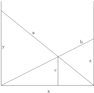
The so-called “Crossed Ladders Problem” can be formulated as follows. Two ladders of lengths a,b, lean against two vertical walls as shown in Figure 1. The ladders cross each other at a point with distance c above the ground. Determine the distance x between the walls and the heights y, z, above the ground of the points where the ladders touch the walls.
The defining system of equations is
x2=a2−y2=b2−z2, (1.1) c= yz
y+z. (1.2)
There is enormous literature on the crossed ladder problem, as may be seen for ex- ample by consulting the extensive bibliography of Singmaster’s “Sources in Recre- ational Mathematics”, Section 6L: “Geometric Recreations. Crossed ladders”; see Singmaster [9]. The second and third authors have also recently investigated this problem; see Høibakk et al. [4, 5].
29