ES ZTERHÁZYKÁROLY
CO LL
EGE
EGER 17 74
Contents
M. Ahmia, H. Belbachir, A. Belkhir, The log-concavity and log-con- vexity properties associated to hyperpell and hyperpell-lucas sequences . 3 S. Bácsó, R. Tornai, Z. Horváth,On geodesic mappings of Riemannian
spaces with cyclic Ricci tensor . . . 13 M. Bahşi, I. Mező, S. Solak,A symmetric algorithm for hyper-Fibonacci
and hyper-Lucas numbers . . . 19 A. Bremner, A. Macleod,An unusual cubic representation problem . . . 29 Chak-On Chow, Shi-Mei Ma, T. Mansour, M. Shattuck, Counting
permutations by cyclic peaks and valleys . . . 43 P. Csiba, F. Filip, A. Komzsík, J. T. Tóth, On the existence of the
generalized Gauss composition of means . . . 55 T. Glavosits, Á. Száz, Divisible and cancellable subsets of groupoids . . . 67 T. Juhász, Commutator identities on group algebras . . . 93 E. Kılıç, Y. T. Ulutaş, I. Akkus, N. Ömür,Generalized binary recurrent
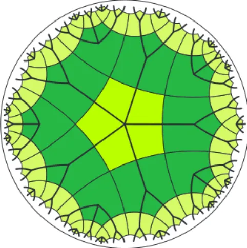
quasi-cyclic matrices . . . 103 L. Németh, L. Szalay, Coincidences in numbers of graph vertices corre-
sponding to regular planar hyperbolic mosaics . . . 113 W. Schreiner, T. Bérczes, J. Sztrik, Probabilistic model checking on
HPC systems for the performance analysis of mobile networks . . . 123 E. Troll,Constrained modification of the cubic trigonometric Bézier curve
with two shape parameters . . . 145 Methodological papers
N. K. Bilan, I. Jelić,On intersections of the exponential and logarithmic curves . . . 159 R. Nagy-Kondor,Importance of spatial visualization skills in Hungary and
Turkey: Comparative Studies . . . 171 P. Szlávi, L. Zsakó, IT Competences: Modelling the Real World . . . 183
ANNALESMATHEMATICAEETINFORMATICAE43.(2014)
TOMUS 43. (2014)
COMMISSIO REDACTORIUM
Sándor Bácsó (Debrecen), Sonja Gorjanc (Zagreb), Tibor Gyimóthy (Szeged), Miklós Hoffmann (Eger), József Holovács (Eger), László Kovács (Miskolc),
László Kozma (Budapest), Kálmán Liptai (Eger), Florian Luca (Mexico), Giuseppe Mastroianni (Potenza), Ferenc Mátyás (Eger),
Ákos Pintér (Debrecen), Miklós Rontó (Miskolc), László Szalay (Sopron), János Sztrik (Debrecen), Gary Walsh (Ottawa)
ANNALES MATHEMATICAE ET INFORMATICAE International journal for mathematics and computer science
Referred by
Zentralblatt für Mathematik and
Mathematical Reviews
The journal of the Institute of Mathematics and Informatics of Eszterházy Károly College is open for scientific publications in mathematics and computer science, where the field of number theory, group theory, constructive and computer aided geometry as well as theoretical and practical aspects of programming languages receive particular emphasis. Methodological papers are also welcome. Papers sub- mitted to the journal should be written in English. Only new and unpublished material can be accepted.
Authors are kindly asked to write the final form of their manuscript in LATEX. If you have any problems or questions, please write an e-mail to the managing editor Miklós Hoffmann: hofi@ektf.hu
The volumes are available athttp://ami.ektf.hu
MATHEMATICAE ET INFORMATICAE
VOLUME 43. (2014)
EDITORIAL BOARD
Sándor Bácsó (Debrecen), Sonja Gorjanc (Zagreb), Tibor Gyimóthy (Szeged), Miklós Hoffmann (Eger), József Holovács (Eger), László Kovács (Miskolc),
László Kozma (Budapest), Kálmán Liptai (Eger), Florian Luca (Mexico), Giuseppe Mastroianni (Potenza), Ferenc Mátyás (Eger),
Ákos Pintér (Debrecen), Miklós Rontó (Miskolc), László Szalay (Sopron), János Sztrik (Debrecen), Gary Walsh (Ottawa)
INSTITUTE OF MATHEMATICS AND INFORMATICS ESZTERHÁZY KÁROLY COLLEGE
HUNGARY, EGER
A kiadásért felelős az Eszterházy Károly Főiskola rektora Megjelent az EKF Líceum Kiadó gondozásában
Kiadóvezető: Czeglédi László Műszaki szerkesztő: Tómács Tibor Megjelent: 2014. december Példányszám: 30
Készítette az
Eszterházy Károly Főiskola nyomdája Felelős vezető: Kérészy László
The log-concavity and log-convexity properties associated to hyperpell and
hyperpell-lucas sequences
Moussa Ahmia
ab, Hacène Belbachir
b, Amine Belkhir
baUFAS, Dep. of Math., DG-RSDT, Setif 19000, Algeria ahmiamoussa@gmail.com
bUSTHB, Fac. of Math., RECITS Laboratory, DG-RSDT, BP 32, El Alia 16111, Bab Ezzouar, Algiers, Algeria hacenebelbachir@gmail.comorhbelbachir@usthb.dz
ambelkhir@gmail.comorambelkhir@usthb.dz Submitted July 22, 2014 — Accepted December 12, 2014
Abstract
We establish the log-concavity and the log-convexity properties for the hyperpell, hyperpell-lucas and associated sequences. Further, we investigate theq-log-concavity property.
Keywords:hyperpell numbers; hyperpell-lucas numbers; log-concavity;q-log- concavity, log-convexity.
MSC:11B39; 05A19; 11B37.
1. Introduction
Zheng and Liu [13] discuss the properties of the hyperfibonacci numbersFn[r] and the hyperlucas numbersL[r]n .They investigate the log-concavity and the log convex- ity property of hyperfibonacci and hyperlucas numbers. In addition, they extend their work to the generalized hyperfibonacci and hyperlucas numbers.
http://ami.ektf.hu
3
Thehyperfibonacci numbers Fn[r] and hyperlucas numbers L[r]n , introduced by Dil and Mező [9] are defined as follows. Put
Fn[r]= Xn k=0
Fk[r−1], with Fn[0]=Fn,
L[r]n = Xn k=0
L[rk−1], with L[0]n =Ln,
whereris a positive integer, andFn andLn are the Fibonacci and Lucas numbers, respectively.
Belbachir and Belkhir [1] gave a combinatorial interpretation and an explicit formula for hyperfibonacci numbers,
Fn+1[r] =
bXn/2c k=0
n+r−k k+r
. (1.1)
Let {Un}n≥0 and {Vn}n≥0 denote the generalized Fibonacci and Lucas se- quences given by the recurrence relation
Wn+1=pWn+Wn−1 (n≥1), with U0= 0, U1= 1, V0= 2, V1=p. (1.2) The Binet forms ofUn andVn are
Un= τn−(−1)nτ−n
√∆ and Vn=τn+ (−1)nτ−n; (1.3) with∆ =p2+ 4, τ= (p+√
∆)/2, andp≥1.
The generalized hyperfibonacci and generalized hyperlucas numbers are defined, respectively, by
Un[r]:=
Xn k=0
Uk[r−1], with Un[0]=Un,
Vn[r] :=
Xn k=0
Vk[r−1], with Vn[0]=Vn.
The paper of Zheng and Liu [13] allows us to exploit other relevant results.
More precisely, we propose some results on log-concavity and log-convexity in the case ofp= 2for the hyperpell sequence and the hyperpell-lucas sequence.
Definition 1.1. Hyperpell numbers Pn[r] and hyperpell-lucas numbers Q[r]n are defined by
Pn[r]:=
Xn k=0
Pk[r−1], with Pn[0]=Pn,
Q[r]n :=
Xn k=0
Q[r−1]k , with Q[0]n =Qn,
where ris a positive integer, and {Pn} and {Qn} are the Pell and the Pell-Lucas sequences respectively.
Now we recall some formulas for Pell and Pell-Lucas numbers. It is well know that the Binet forms ofPn andQn are
Pn =αn−(−1)nα−n 2√
2 and Qn=αn+ (−1)nα−n, (1.4) whereα= (1 +√
2). The integers P(n, k) = 2n−2k
n−k k
and Q(n, k) = 2n−2k n n−k
n−k k
, (1.5) are linked to the sequences{Pn}and{Qn}.It is established [2] that for each fixed nthese two sequences are log-concave and then unimodal. For the generalized se- quence given by(1.2),also the corresponding associated sequences are log-concave and then unimodal, see [3, 4].
The sequences{Pn} and {Qn} satisfy the recurrence relation (1.2), for p= 2, and forn≥0 andn≥1respectively, we have
Pn+1=
bXn/2c k=0
2n−2k n−k
k
and Qn=
bXn/2c k=0
2n−2k n n−k
n−k k
. (1.6) It follows from (1.4) that the following formulas hold
Pn2−Pn−1Pn+1= (−1)n+1, (1.7) Q2n−Qn−1Qn+1= 8(−1)n. (1.8) It is easy to see, for example by induction, that forn≥1
Pn≥n and Qn≥n. (1.9)
Let{xn}n≥0 be a sequence of nonnegative numbers. The sequence{xn}n≥0 is log-concave(respectivelylog-convex) ifx2j ≥xj−1xj+1(respectivelyx2j ≤xj−1xj+1
) for all j > 0, which is equivalent (see [5]) to xixj ≥ xi−1xj+1 (respectively xixj ≤xi−1xj+1) forj≥i≥1.
We say that{xn}n≥0 islog-balanced if{xn}n≥0 is log-convex and {xn/n!}n≥0
is log-concave.
Letq be an indeterminate and{fn(q)}n≥0 be a sequence of polynomials ofq.
If for eachn≥1, fn2(q)−fn−1(q)fn+1(q)has nonnegative coefficients,we say that {fn(q)}n≥0 isq-log-concave.
In section 2, we give the generating functions of hyperpell and hyperpell-lucas sequences. In section 3, we discuss their log-concavity and log-convexity. We investigate also the q-log-concavity of some polynomials related to hyperpell and hyperpell-lucas numbers.
2. The generating functions
The generating function of Pell numbers and Pell-Lucas numbers denoted GP(t) andGQ(t), respectively, are
GP(t) :=
+∞X
n=0
Pntn= t
1−2t−t2, (2.1)
and
GQ(t) :=
+∞X
n=0
Qntn= 2−2t
1−2t−t2. (2.2)
So, we establish the generating function of hyperpell and hyperpell-lucas num- bers using respectively
Pn[r] =Pn−1[r] +Pn[r−1] and Q[r]n =Q[r]n−1+Q[rn−1]. (2.3) The generating functions of hyperpell numbers and hyperlucas numbers are
G[r]P (t) = X∞ n=0
Pn[r]tn= t
(1−2t−t2) (1−t)r, (2.4) and
G[r]Q(t) = X∞ n=0
Q[r]n tn= 2−2t
(1−2t−t2) (1−t)r. (2.5)
3. The log-concavity and log-convexity properties
We start the section by some useful lemmas.
Lemma 3.1. [12]If the sequences{xn} and{yn} are log-concave, then so is their ordinary convolutionzn=Pn
k=0xkyn−k, n= 0,1, ....
Lemma 3.2. [12] If the sequence {xn} is log-concave, then so is the binomial convolution zn=Pn
k=0 n k
xk, n= 0,1, ....
Lemma 3.3. [8]If the sequence {xn} is log-convex, then so is the binomial con- volution zn=Pn
k=0 n k
xk, n= 0,1, ....
The following result deals with the log-concavity of hyperpell numbers and hyperlucas sequences.
Theorem 3.4. The sequencesn Pn[r]
o
n≥0andn Q[r]n
o
n≥0 are log-concave forr≥1 andr≥2 respectively.
Proof. We have
Pn[1]= 1
4(Qn+1−2) and Q[1]n = 2Pn+1. (3.1) Whenn= 1,
Pn[1]
2
−Pn[1]−1Pn+1[1] = 1>0. Whenn≥2,it follows from(3.1) and(1.8)that
Pn[1]2
−Pn[1]−1Pn+1[1] = 1 16
h(Qn+1−2)2−(Qn−2) (Qn+2−2)i
= 1
16 Q2n+1−QnQn+2−4Qn+1+ 2Qn+ 2Qn+2
= 1
4 2(−1)n−1+Qn+1
≥0.
Then n Pn[1]
o
n≥0 is log-concave. By Lemma 3.1, we know that n Pn[r]
o
n≥0
(r≥1)is log-concave.
It follows from(3.1)and(1.7)that Q[1]n 2
−Q[1]n−1Q[1]n+1= 4 Pn+12 −PnPn+2
= 4 (−1)n=±4 (3.2) Hencen
Q[1]n
o
n≥0 is not log-concave.
One can verify that
Q[2]n = 1
2(Qn+2−2) = 2Pn+1[1] . (3.3) Then n
Q[2]n
o
n≥0 is log-concave. By Lemma 3.1, we know that n Q[r]n
o
n≥0
(r≥2)is log-concave. This completes the proof of Theorem3.4.
Then we have the following corollary.
Corollary 3.5. The sequences nPn k=0
n k
Pk[r]o
n≥0 and nPn k=0
n k
Q[r]k o
n≥0 are log-concave forr≥1 andr≥2 respectively.
Proof. Use Lemma 3.2.
Now we establish thelog-concavity of order twoof the sequencesn Pn[1]
o
n≥0and nQ[2]n
o
n≥0 for some special sub-sequences.
Theorem 3.6. Let be for n≥1 Tn:=
Pn[1]2
−Pn[1]−1Pn+1[1] and Rn:=
Q[2]n 2
−Q[2]n−1Q[2]n+1.
Then{T2n}n≥1,{R2n+1}n≥0 are log-concave, and{T2n+1}n≥0,{R2n}n≥1 are log- convex.
Proof. Using respectively(3.3)and (1.8),we get Q[2]n 2
−Q[2]n−1Q[2]n+1= 2(−1)n+Qn+1, and thus, forn≥1,
Tn= 1 4
2 (−1)n−1+Qn
and Rn= 2(−1)n+Qn+1. (3.4)
By applying(3.4) and(1.8), forn≥1 we get
Q22n−Q2n−2Q2n+2=−32 and Q22n+1−Q2n−1Q2n+3= 32. (3.5) Then
T2n2 −T2(n−1)T2(n+1)= 1
16 Q22n−Q2n−2Q2n+2−4Q2n+ 2Q2n−2+ 2Q2n+2
= 4(Q2n−4)>0.
and
R22n+1−R2n−1R2n+3= Q22n+2−Q2nQ2n+2−4Q2n+2+ 2Q2n+ 2Q2n+4
= 64(Q2n+2−4)>0.
Then{T2n}n≥1 and{R2n+1}n≥0 are log-concave.
Similarly by applying (3.4) and (3.5), we have T2n+12 −T2n−1T2n+3=−1
2Q2n+1<0, and
R22n−R2(n−1)R2(n+1)=−8Q2n+1<0.
Then{T2n+1}n≥0 and{R2n}n≥1 are log-convex. This completes the proof.
Corollary 3.7. The sequences Pn k=0
n k
T2k n≥0 andPn k=0
n k
R2k+1 n≥0 are log-concave.
Proof. Use Lemma 3.2.
Corollary 3.8. The sequences Pn k=0
n k
T2k+1 n≥1 and Pn k=0
n k
R2k n≥1 are log-convex.
Proof. Use Lemma 3.3.
Lemma 3.9. Let an:=Pn k=0
n k
Pk+1,where{Pn}n≥0 is the Pell sequence. Then {an}n≥0 satisfy the following recurrence relations
an= 3an−1+
n−2
X
k=0
ak and an= 4an−1−2an−2.
Proof. Let be bn := Pn k=0
n k
Pk, where {Pn}n≥−1 is the Pell sequence extended toP−1= 1.
Using Pascal formula and the recurrence relation of Pell sequence together into the development Pn
k=0 n k
Pk+1 we getan = 3an−1+bn−1, then by bn =bn−1+ an−1. By iterated use of this relation with the precedent one, we getan= 3an−1+ Pn−2
k=0ak (withb0= 0 anda0= 1), thusan= 4an−1−2an−2. Theorem 3.10. The sequences n
nQ[1]n
o
n≥0 and nPn k=0
n k
Q[1]k o
n≥0 are log- concave and log-convex, respectively.
Proof. Let be Sn:=n2
Q[1]n 2
−(n2−1)Q[1]n−1Q[1]n+1 and Kn:=
Xn k=0
n k
Q[1]k , with the convention thatK<0= 0.
From (3.2), we have
Sn= 4(n2−1) (−1)n+ Q[1]n 2
= 4
(n2−1) (−1)n+Pn+12
≥4
(n2−1) (−1)n+ (n+ 1)2
>0.
Thenn nQ[1]n
o
n≥0 is log-concave.
Using Lemma3.9,we can verify that
Kn= 4Kn−1−2Kn−2. (3.6)
The associated Binet-formula is Kn= 1 +√
2
αn− 1−√ 2
βn
α−β , with α, β= 2±√ 2, which provides
Kn2−Kn−1Kn+1=−2n+1<0.
ThennPn k=0
n k
Q[1]k o
n≥0 is log-convex.
Remark 3.11. The terms of the sequence{Kn}n satisfyKn= 2(n+2)/2Pn+1 ifnis even, and Kn = 2(n−1)/2Qn+1 ifnis odd.
Theorem 3.12. The sequences n n!Pn[1]
o
n≥0 andn n!Q[2]n
o
n≥0 are log-balanced.
Proof. By Theorem 3.4, in order to prove the log-balanced property ofn n!Pn[1]
o
n≥0
and n n!Q[2]n
o
n≥0 we only need to show that they are log-convex. It follows from the proof of Theorem 3.4 that
Pn[1]2
−Pn−1[1] Pn+1[1] =1 4
2 (−1)n−1+Qn+1
, (3.7)
and from the proof of Theorem 3.6 that Q[2]n 2
−Q[2]n−1Q[2]n+1= 2 (−1)n+Qn+1. (3.8) Let
Mn :=n Pn[1]2
−(n+ 1)Pn[1]−1Pn+1[1] , Bn :=n
Q[2]n 2
−(n+ 1)Q[2]n−1Q[2]n+1, from (3.3), (3.7) and (3.8), we get
Mn =(n+ 1) 4
2 (−1)n−1+Qn+1
−1
4(Qn+1−2)2, Bn = (n+ 1) (2 (−1)n+Qn+1)−1
4(Qn+2−2)2.
ClearlyBn ≤0for n= 0,1,2. We have by induction that forn≥1, Qn ≥n+ 1.
This gives
Bn≤(Qn+1−1) (2 (−1)n+Qn+1)−1
4(2Qn+1+Qn−2)2<0.
Also,Mn ≤0for n= 2and forn≥3, Qn ≥n+ 6.This givesn+ 1≤Qn+1−6, and
Mn≤ 1 4
h(Qn+1−6)
2 (−1)n−1+Qn+1
−(Qn+1−2)2i
= 1 4
h−2 + 2 (−1)n−1
Qn+1−4−12 (−1)n−1i
<0.
Hence {n!Pn[1]}n≥0 and {n!Q[2]n }n≥0 are log-convex. As the sequences {Pn[1]}n≥0
and {Q[2]n }n≥0 are log-concave, so the sequences{n!Pn[1]}n≥0 and{n!Q[2]n }n≥0 are log-balanced.
Theorem 3.13. Define, for r≥1, the polynomials Pn,r(q) :=
Xn k=0
Pk[r]qk and Qn,r(q) :=
Xn k=0
Q[r]k qk. The polynomialsPn,r(q) (r≥1)andQn,r(q) (r≥2)are q-log-concave.
Proof. Whenn≥1, r≥1,
Pn,r2 (q)−Pn−1,r(q)Pn+1,r(q)
= Xn k=0
Pk[r]qk
!2
−
n−1X
k=0
Pk[r]qk
! n+1 X
k=0
Pk[r]qk
!
= Xn k=0
Pk[r]qk
!2
− Xn k=0
Pk[r]qk−Pn[r]qn
! n X
k=0
Pk[r]qk+Pn+1[r] qn+1
!
=
Pn[r]qn−Pn+1[r] qn+1Xn
k=0
Pk[r]qk+Pn[r]Pn+1[r] q2n+1
= Xn k=1
Pk[r]Pn[r]−Pk−1[r] Pn+1[r]
qk+n.
Whenn≥1, r≥2, through computation, we get Q2n,r(q)−Qn−1,r(q)Qn+1,r(q) =
Xn k=1
Q[r]k Q[r]n −Q[r]k−1Q[r]n+1
qk+n+Q[r]n qn. As n
Pn[r]
o and n Q[r]n
o (r≥2) are log-concave, then the polynomials Pn,r(q) (r≥1)and Qn,r(q) (r≥2)areq-log-concave.
Acknowledgements. We would like to thank the referee for useful suggestions and several comments witch involve the quality of the paper.
References
[1] Belbachir, H., Belkhir, A., Combinatorial Expressions Involving Fibonacci, Hy- perfibonacci, and Incomplete Fibonacci Numbers, J. Integer Seq., Vol. 17 (2014), Article 14.4.3.
[2] Belbachir, H., Bencherif, F., Unimodality of sequences associated to Pell num- bers,Ars Combin.,102 (2011), 305–311.
[3] Belbachir, H., Bencherif, F., Szalay, L., Unimodality of certain sequences connected with binomial coefficients, J. Integer Seq.,10 (2007), Article 07. 2. 3.
[4] Belbachir, H., Szalay, L., Unimodal rays in the regular and generalized Pascal triangles,J. Integer Seq.,11 (2008), Article. 08.2.4.
[5] Brenti, F., Unimodal, log-concave and Pólya frequency sequences in combinatorics, Mem. Amer. Math. Soc.,no. 413 (1989).
[6] Cao, N. N., Zhao, F. Z, Some Properties of Hyperfibonacci and Hyperlucas Num- bers,J. Integer Seq.,13 (8) (2010), Article 10.8.8.
[7] Chen, W. Y. C., Wang, L. X. W., Yang, A. L. B., Schur positivity and the q-log-convexity of the Narayana polynomials,J. Algebr. Comb.,32 (2010), 303–338.
[8] Davenport, H., Pólya, G., On the product of two power series, Canadian J.
Math.,1 (1949), 1–5.
[9] Dil, A., Mező, I., A symmetric algorithm for hyperharmonic and Fibonacci num- bers,Appl. Math. Comput.,206 (2008), 942–951.
[10] Liu, L., Wang, Y., On the log-convexity of combinatorial sequences, Advances in Applied Mathematics,vol. 39, Issue 4, (2007), 453–476.
[11] Sloane, N. J. A., On-line Encyclopedia of Integer Sequences, http://oeis.org, (2014).
[12] Wang, Y., Yeh, Y. N., Log-concavity and LC-positivity,Combin. Theory Ser. A, 114 (2007), 195–210.
[13] Zheng, L. N., Liu, R., On the Log-Concavity of the Hyperfibonacci Numbers and the Hyperlucas Numbers,J. Integer Seq.,Vol. 17 (2014), Article 14.1.4.
On geodesic mappings of Riemannian spaces with cyclic Ricci tensor
Sándor Bácsó
a, Robert Tornai
a, Zoltán Horváth
baUniversity of Debrecen, Faculty of Informatics bacsos@unideb.hu,tornai.robert@inf.unideb.hu
bFerenc Rákóczi II. Transcarpathian Hungarian Institute zolee27@kmf.uz.ua
Submitted May 4, 2012 — Accepted March 25, 2014
Abstract
An n-dimensional Riemannian space Vn is called a Riemannian space with cyclic Ricci tensor [2, 3], if the Ricci tensorRij satisfies the following condition
Rij,k+Rjk,i+Rki,j= 0,
whereRij the Ricci tensor ofVn, and the symbol ”,” denotes the covariant derivation with respect to Levi-Civita connection ofVn.
In this paper we would like to treat some results in the subject of geodesic mappings of Riemannian space with cyclic Ricci tensor.
Let Vn = (Mn, gij) and Vn = (Mn, gij) be two Riemannian spaces on the underlying manifoldMn. A mappingVn →Vnis called geodesic, if it maps an arbitrary geodesic curve ofVnto a geodesic curve ofVn.[4]
At first we investigate the geodesic mappings of a Riemannian space with cyclic Ricci tensor into another Riemannian space with cyclic Ricci tensor.
Finally we show that, the Riemannian - Einstein space with cyclic Ricci tensor admit only trivial geodesic mapping.
Keywords:Riemannian spaces, geodesic mapping.
MSC:53B40.
http://ami.ektf.hu
13
1. Introduction
Let an n-dimensionalVn Riemannian space be given with the fundamental tensor gij(x). Vn has the Riemannian curvature tensorRijkl in the following form:
Rhijk(x) =∂jΓhik(x) + Γαik(x)Γhjα(x)−∂kΓhij(x)−Γαij(x)Γhkα(x), (1.1) whereΓijk(x)are the coefficients of Levi-Civita connection ofVn.
The Ricci curvature tensor we obtain from the Riemannian curvature tensor using of the following transvection: Rαjkα(x) =Rjk(x)1.
Definition 1.1. [2, 3] A Riemannian spaceVn is called a Riemannian space with cyclic Ricci tensor, if the Ricci tensor ofVn satisfies the following equation:
Rij,k+Rjk,i+Rki,j = 0, (1.2) where the symbol ”,” means the covariant derivation with respect to Levi-Civita connection ofVn.
Definition 1.2. [4] Let two Riemannian spaces Vn andVn be given on the un- derlying manifold Mn . The maps: γ : Vn → Vn is called geodesic (projective) mappings, if any geodesic curve ofVn coincides with a geodesic curve ofVn.
It is wellknown, that the the geodesic curvexi(t)ofVnis a result of the second order ordinary differential equations in a canonical parameter t:
d2xi
dt2 + Γiαβ(x)dxα dt
dxβ
dt = 0. (1.3)
We need in the investigations the next:
Theorem 1.3. [4] The maps: Vn→Vn is geodesic if and only if exits a gradient vector fieldψi(x), which satisfies the following condition:
Γijk(x) = Γijk(x) +δjiψk(x) +δikψj(x), (1.4) and
Definition 1.4. [1] A Riemannian space Vn is called Einstein space, if exists a ρ(x)scalar function, which satisfies the equation:
Rij =ρ(x)gij(x). (1.5)
1The Roman and Greek indices run over the range 1, . . . , n; the Roman indices are free but the Greek indices denote summation.
2. Geodesic mappings of Riemannian spaces with cyclic Ricci tensors
It is easy to get the next equations [4]:
Rij =Rij+ (n−1)ψij, (2.1)
whereψij =ψi,j−ψiψj and Rij,k= ∂Rij
∂xk −Γαik(x)Rαj−Γαjk(x)Rαi, (2.2) whereΓαik(x)are components of Levi-Civita connection ifVn.
At now we suppose, that Vn in a Riemannian space with cyclic Ricci tensor, that is
Rij,k+Rjk,i+Rki,j = 0. (2.3) Using (2.2) we can rewrite (2.3) in the following form:
∂Rij
∂xk −Γαik(x)Rαj−Γαjk(x)Rαi+
∂Rjk
∂xi −Γαji(x)Rαk−Γαki(x)Rαj+
∂Rki
∂xj −Γαkj(x)Rαi−Γαij(x)Rαk= 0.
(2.4)
From (1.4) and (2.1) we can compute:
∂(Rij+ (n−1)ψij)
∂xk −(Γαik(x) +ψi(x)δαk +ψk(x)δiα)(Rαj+ (n−1)ψαj)−
−(Γαjk(x) +ψj(x)δαk +ψk(x)δαj)(Rαi+ (n−1)ψαi)+
∂(Rjk+ (n−1)ψjk)
∂xi −(Γαji(x) +ψj(x)δiα+ψi(x)δjα)(Rαk+ (n−1)ψαk)−
−(Γαki(x) +ψk(x)δiα+ψi(x)δkα)(Rαj+ (n−1)ψαj)+
∂(Rki+ (n−1)ψki)
∂xj −(Γαkj(x) +ψk(x)δjα+ψj(x)δαk)(Rαi+ (n−1)ψαi)−
−(Γαij(x) +ψi(x)δαj +ψj(x)δiα)(Rαk+ (n−1)ψαk) = 0.
That is
∂Rij
∂xk −Γαik(x)Rαj−Γαjk(x)Rαi+ +∂R∂xjki −Γαji(x)Rαk−Γαki(x)Rαj+ +∂R∂xkij −Γαkj(x)Rαi−Γαij(x)Rαk+
Rij,k+Rjk,i+Rki,j
+(n−1)∂ψij
∂xk −(n−1)Γαik(x)ψαj−ψi(x)Rkj−(n−1)ψi(x)ψkj−
−ψk(x)Rij−(n−1)ψk(x)ψij−(n−1)Γαjk(x)ψαi−ψj(x)Rki−
−(n−1)ψj(x)ψki−ψk(x)Rji−(n−1)ψk(x)ψji+ +(n−1)∂ψjk
∂xi −(n−1)Γαji(x)ψαk−ψj(x)Rik−(n−1)ψj(x)ψik−
−ψi(x)Rjk−(n−1)ψi(x)ψjk−(n−1)Γαki(x)ψαj−ψk(x)Rij−
−(n−1)ψk(x)ψij−ψi(x)Rkj−(n−1)ψi(x)ψkj+ +(n−1)∂ψki
∂xj −(n−1)Γαkj(x)ψαi−ψk(x)Rji−(n−1)ψk(x)ψji−
−ψj(x)Rki−(n−1)ψj(x)ψki−(n−1)Γαij(x)ψαk−ψi(x)Rjk−
−(n−1)ψi(x)ψjk−ψj(x)Rik−(n−1)ψj(x)ψik= 0.
If we suppose, thatVn has cyclic Ricci tensor we have:
(n−1) ∂ψij
∂xk −Γαik(x)ψαj−Γαjk(x)ψαi
+
+(n−1) ∂ψjk
∂xi −Γαji(x)ψαk−Γαki(x)ψαj
+ +(n−1)
∂ψki
∂xj −Γαkj(x)ψαi−Γαij(x)ψαk
+
−4ψi(x)Rjk−4ψj(x)Rki−4ψk(x)Rij−
−(n−1)(4ψi(x)ψjk+ 4ψj(x)ψki+ 4ψk(x)ψij) = 0.
That is
(n−1)(ψij,k+ψjk,i+ψki,j)−
−4(ψi(x)Rjk+ψj(x)Rki+ψk(x)Rij)−
−4(n−1)(ψi(x)ψjk+ψj(x)ψki+ψk(x)ψij) = 0.
(2.5)
Theorem 2.1. VnandVn Riemannian spaces with cyclic Ricci tensors have com- mon geodesics, that isVn and Vn have a geodesic mapping if and only if exists a ψi(x)gradient vector, which satisfies the condition:
(n−1)(ψij,k+ψjk,i+ψki,j)−
−4(ψi(x)Rjk+ψj(x)Rki+ψk(x)Rij)−
−4(n−1)(ψi(x)ψjk+ψj(x)ψki+ψk(x)ψij) = 0.
3. Consequences
A) Ifψij = 0, thenRij=Rij, andψi,j=ψiψj, so we obtain:
ψi(x)Rjk+ψj(x)Rki+ψk(x)Rij = 0. (3.1) B) If theVn is a Riemannian space with cyclic Ricci tensor and at the same time is a Einstein space, then we get
ρψi(x)gjk+ρψj(x)gki+ρψk(x)gij= 0 that is
nψi(x) + 2ψi(x) = 0, (3.2) so
(n+ 2)ψi(x) = 0. (3.3)
It means
Theorem 3.1. A Riemannian-Einstein space Vn with cyclic Ricci tensor admits intoVn with cyclic Ricci tensor only trivial (affin) geodesic mapping.
References
[1] A. L. Besse, Einstein manifolds,Springer-Verlag, (1987)
[2] T. Q. Binh, On weakly symmetric Riemannian spaces,Publ. Math. Debrecen, 42/1-2 (1993), 103–107.
[3] M. C. Chaki - U. C. De, On pseudo symmetric spaces,Acta Math. Hung., 54 (1989), 185–190.
[4] N. Sz. Szinjukov, Geodezicseszkije otrobrazsenyija Rimanovih prosztransztv, Moscow, Nauka, (1979)
A symmetric algorithm for hyper-Fibonacci and hyper-Lucas numbers
Mustafa Bahşi
a, István Mező
b∗, Süleyman Solak
caAksaray University, Education Faculty, Aksaray, Turkey mhvbahsi@yahoo.com
bNanjing University of Information Science and Technology, Nanjing, P. R. China istvanmezo81@gmail.com
cN. E. University, A.K Education Faculty, 42090, Meram, Konya, Turkey ssolak42@yahoo.com
Submitted July 22, 2014 — Accepted November 14, 2014
Abstract
In this work we study some combinatorial properties of hyper-Fibonacci, hyper-Lucas numbers and their generalizations by using a symmetric algo- rithm obtained by the recurrence relation akn =uakn−1+vakn−1. We point out that this algorithm can be applied to hyper-Fibonacci, hyper-Lucas and hyper-Horadam numbers.
Keywords:Hyper-Fibonacci numbers; hyper-Lucas numbers MSC:11B37; 11B39; 11B65
1. Introduction
The sequence of Fibonacci numbers is one of the most well known sequence, and it has many applications in mathematics, statistics, and physics. The Fibonacci numbers are defined by the second order linear recurrence relation: Fn+1=Fn+ Fn−1 (n≥1) with the initial conditionsF0 = 0andF1 = 1. Similarly, the Lucas
∗The research of István Mező was supported by the Scientific Research Foundation of Nanjing University of Information Science & Technology, and The Startup Foundation for Introducing Talent of NUIST. Project no.: S8113062001
http://ami.ektf.hu
19
numbers are defined by Ln+1 = Ln +Ln−1 (n≥1) with the initial conditions L0 = 2 and L1 = 1. There are some elementary identities for Fn and Ln. Two of them areFs+ Ls = 2Fs+1 and Fs−Ls = 2Fs−1. These will be generalized in section 2 (see Theorem 2.5).
The Fibonacci sequence can be generalized to the second order linear recurrence Wn(a, b;p, q),or brieflyWn,defined by
Wn+1=pWn+qWn−1,
where n≥1, W0=aandW1=b.This sequence was introduced by Horadam [7].
Some of the special cases are:
i) The Fibonacci numberFn=Wn(0,1; 1,1), ii) The Lucas numberLn=Wn(2,1; 1,1), iii) The Pell numberPn=Wn(0,1; 2,1).
In [4], Dil and Mező introduced the “hyper-Fibonacci” numbersFn(r)and “hyper- Lucas” numbersL(r)n . These are defined as
Fn(r)= Xn k=0
Fk(r−1) with Fn(0)=Fn, F0(r)= 0, F1(r)= 1,
L(r)n = Xn k=0
L(r−1)k with L(0)n =Ln, L(r)0 = 2, L(r)1 = 2r+ 1,
where ris a positive integer, moreoverFn andLn are the ordinary Fibonacci and Lucas numbers, respectively. The generating functions of hyper-Fibonacci and hyper-Lucas numbers are [4]:
X∞ n=0
Fn(r)tn = t
(1−t−t2) (1−t)r, X∞ n=0
L(r)n tn= 2−t
(1−t−t2) (1−t)r. Also, the hyper-Fibonacci and hyper-Lucas numbers have the recurrence relations Fn(r)=Fn(r)−1+Fn(r−1)andL(r)n =L(r)n−1+L(rn−1), respectively. The first few values ofFn(r) andL(r)n are as follows [2]:
Fn(1): 0,1,2,4,7,12,20,33,54, . . . , Fn(2): 0,1,3,7,14,26,46,79, . . . L(1)n : 2,3,6,10,17,28,46,75, . . . , L(2)n : 2,5,11,21,38,66,112, . . . .
Now we introduce the hyper-Horadam numbersWn(r)defined by Wn(r)=Wn(r)−1+Wn(r−1) with Wn(0)=Wn, W0(n)=W0=a
whereWnis thenth Horadam number. Some of the special cases of hyper-Horadam number Wn(r) are as follows:
i) If Wn(0) =Fn =Wn(0,1; 1,1) and W0(n) =W0 =F0= 0, thenWn(r) is the hyper-Fibonacci number, that is,Wn(r)=Fn(r).
ii) If Wn(0) =Ln =Wn(2,1; 1,1) andW0(n) =W0 =L0 = 2, thenWn(r) is the hyper-Lucas number, that is,Wn(r)=L(r)n .
iii) IfWn(0) =Pn =Wn(0,1; 2,1) and W0(n) =W0 =P0 = 0, then Wn(r) is the hyper-Pell number, that is,Wn(r)=Pn(r).
The paper is organized as follows: In Section 2 we give some combinatorial properties of the hyper-Fibonacci and hyper-Lucas numbers by using a symmetric algorithm. In Section 3 we generalize the symmetric algorithm introduced in section 2 and, in addition, we generalize the hyper-Horadam numbers as well.
2. A symmetric algorithm
The Euler–Seidel algorithm and its analogues are useful in the study of recurrence relations of some numbers and polynomials [2, 3, 4, 5]. Let(an)and(an)be two real initial sequences. Then the infinite matrix, which is called symmetric infinite matrix in [4], with entriesakn corresponding to these sequences is determined recursively by the formulas
a0n=an, an0 =an (n≥0), akn=ak−1n +akn−1 (n≥1, k≥1), i.e., in matrix form
. . . .
. . . .
. . . .
. . . . ak−1n
↓
. . . . . . akn−1→ akn . . .
. . . .
. . . .
. . . .
.
The entriesakn (wherekis the row index,nis the column index) have the following symmetric relation [4]:
akn= Xk i=1
n+k−i−1 n−1
ai0+
Xn s=1
n+k−s−1 k−1
a0s. (2.1) Dil and Mező [4], by using the relation (2.1), obtained an explicit formula for hyperharmonic numbers, general generating functions of the Fibonacci and Lucas
numbers. By using relation (2.1) and the following well known identity [6, p. 160]
Xc t=a
t a
= c+ 1
a+ 1
, (2.2)
we have some new findings contained in the following theorems.
Theorem 2.1. If n≥1, r≥1 andm≥0,then Fn(m+r)=
Xn s=0
n+r−s−1 r−1
Fs(m).
Proof. Leta0n=Fn+1(m)andan0 =F1(m+n)= 1be given forn≥1. If we calculate the elements of the corresponding infinite matrix by using the recursive formula (2.1), it turns out that they equal to
F1(m) F2(m) F3(m) F4(m) . . . F1(m+1) F2(m+1) F3(m+1) F4(m+1) . . . F1(m+2) F2(m+2) F3(m+2) F4(m+2) . . .
... ... ... ... ...
. (2.3)
From relation (2.1) it follows that ar+1n+1=
Xr+1 i=1
n+r−i+ 1 n
+
n+1X
s=1
n+r−s+ 1 r
Fs+1(m)
= Xr i=0
n+r−i n
+
Xn s=0
n+r−s r
Fs+2(m)
= Xr k=0
n+k n
+
Xn b=0
r+b r
Fn−b+2(m) , wherek=r−iandb=n−s.From (2.2), we have
ar+1n+1=
n+r+ 1 n+ 1
+
Xn b=0
r+b r
Fn−b+2(m) =
n+1X
b=0
r+b r
Fn−b+2(m) . Then the matrix (2.3) yields
arn−1=Fn(m+r)=
n−1
X
b=0
r+b−1 r−1
Fn(m)−b = Xn s=0
n+r−s−1 r−1
Fs(m). Thus the proof is completed.
We then can easily deduce an expression for the hyper-Fibonacci numbers which contains the ordinary Fibonacci numbers.
Corollary 2.2. If n≥1 andr≥1, then Fn(r)=
Xn s=0
n+r−s−1 r−1
Fs
whereFs is thesth Fibonacci number.
The corresponding theorem for the hyper-Lucas numbers is as follows.
Theorem 2.3. If n≥1, r≥1 andm≥0,then L(m+r)n =
Xn s=0
n+r−s−1 r−1
L(m)s .
Proof. Leta0n =L(m)n and an0 =L(m+n)0 = 2be given forn≥1. This special case gives the following infinite matrix:
L(m)0 L(m)1 L(m)2 L(m)3 . . . L(m+1)0 L(m+1)1 L(m+1)2 L(m+1)3 . . . L(m+2)0 L(m+2)1 L(m+2)2 L(m+2)3 . . .
... ... ... ... ...
. (2.4)
From the relation (2.1) we get that
arn= Xr i=1
n+r−i−1 n−1
2 +
Xn s=1
n+r−s−1 r−1
L(m)s
= 2 Xr−1 i=0
n+r−i−2 n−1
+
n−1X
s=0
n+r−s−2 r−1
L(m)s+1
= 2 Xr−1 k=0
n+k−1 n−1
+
n−1X
b=0
r+b−1 r−1
L(m)n−b, wherek=r−i−1andb=n−s−1.From (2.2), we have
arn= 2
n+r−1 n
+
n−1X
b=0
r+b−1 r−1
L(m)n−b = Xn b=0
r+b−1 r−1
L(m)n−b. Then the matrix (2.4) yields
arn=L(m+r)n = Xn b=0
r+b−1 r−1
L(m)n−b = Xn s=0
n+r−s−1 r−1
L(m)s , this completes the proof.
Corollary 2.4. If n≥1 andr≥1, then L(r)n =
Xn s=0
n+r−s−1 r−1
Ls, whereLn is thenth Lucas number.
Theorem 2.5. If n≥1 andr≥1,then i) Fn(r)+L(r)n = 2Fn+1(r) ,
ii) Fn(r)−L(r)n = 2Fn+1(r−1).
Proof. From Corollaries 2.2 and 2.4, we have Fn(r)+L(r)n =
Xn s=0
n+r−s−1 r−1
(Fs+Ls)
= Xn s=0
n+r−s−1 r−1
(2Fs+1) = 2Fn+1(r) and
Fn(r)−L(r)n = Xn s=0
n+r−s−1 r−1
(Fs−Ls)
= Xn s=0
n+r−s−1 r−1
(2Fs−1) = 2Fn+1(r−1). Theorem 2.6. If n≥1 andr≥1,then
Xr s=0
Fn(s)=Fn+1(r) −Fn−1. Proof. From Corollary 2.2, we have
Xr s=1
Fn(s)= Xr s=1
Xn t=0
n+s−t−1 s−1
Ft
!
= Xn t=0
Ft
Xr s=1
n+s−t−1 s−1
! . From (2.2), we obtain
Xr s=1
Fn(s)= Xn t=0
n+r−t r−1
Ft=
n+1X
t=0
n+r−t r−1
Ft−Fn+1=Fn+1(r) −Fn+1.
Thus r
X
s=0
Fn(s)=Fn+1(r) −Fn−1.


![Figure 2: Performance Measures Without Renting (cf. Fig. 2 from [4])](https://thumb-eu.123doks.com/thumbv2/9dokorg/1208488.90412/129.722.95.630.86.635/figure-performance-measures-renting-cf-fig.webp)
![Figure 3: Performance Measures for t 2 = 6 (cf. Fig. 3 from [4])](https://thumb-eu.123doks.com/thumbv2/9dokorg/1208488.90412/130.722.98.626.159.839/figure-performance-measures-t-cf-fig.webp)
![Figure 4: Further Performance Measures for t 2 = 6 (cf. Fig. 4 from [4])](https://thumb-eu.123doks.com/thumbv2/9dokorg/1208488.90412/131.722.96.627.88.460/figure-performance-measures-t-cf-fig.webp)
![Figure 5: Performance Measures for ρ 0 = 0.6 (cf. Fig. 5 from [4])](https://thumb-eu.123doks.com/thumbv2/9dokorg/1208488.90412/132.722.97.626.244.749/figure-performance-measures-ρ-cf-fig.webp)
![Figure 7: AP R vs. t 1 and d for ρ 0 = 4.6 (cf. Fig. 7 from [4])](https://thumb-eu.123doks.com/thumbv2/9dokorg/1208488.90412/133.722.178.547.572.817/figure-ap-r-vs-t-ρ-cf-fig.webp)
