Annales Mathematicae et Informaticae (48.)

(1)

ANNALES

MATHEMATICAE ET INFORMATICAE

TOMUS 48. (2018)

COMMISSIO REDACTORIUM

Sándor Bácsó (Debrecen), Sonja Gorjanc (Zagreb), Tibor Gyimóthy (Szeged), Miklós Hoffmann (Eger), József Holovács (Eger), Tibor Juhász (Eger), László Kovács (Miskolc), László Kozma (Budapest), Kálmán Liptai (Eger), Florian Luca (Mexico), Giuseppe Mastroianni (Potenza), Ferenc Mátyás (Eger),

Ákos Pintér (Debrecen), Miklós Rontó (Miskolc), László Szalay (Sopron), János Sztrik (Debrecen), Gary Walsh (Ottawa)

HUNGARIA, EGER

Annales Mathematicae et Informaticae borító külső oldala

(2)

ANNALES MATHEMATICAE ET INFORMATICAE International journal for mathematics and computer science

Referred by

Zentralblatt für Mathematik and

Mathematical Reviews

The journal of the Institute of Mathematics and Informatics of Eszterházy Károly University of Applied Sciences is open for scientific publications in mathematics and computer science, where the field of number theory, group theory, constructive and computer aided geometry as well as theoretical and practical aspects of programming languages receive particular emphasis. Methodological papers are also welcome. Papers submitted to the journal should be written in English. Only new and unpublished material can be accepted.

Authors are kindly asked to write the final form of their manuscript in L^ATEX. If you have any problems or questions, please write an e-mail to the managing editor Miklós Hoffmann: hofi@ektf.hu

The volumes are available athttp://ami.uni-eszterhazy.hu

Annales Mathematicae et Informaticaeborító belső oldala

(3)

ANNALES

MATHEMATICAE ET INFORMATICAE

VOLUME 48. (2018)

EDITORIAL BOARD

Sándor Bácsó (Debrecen), Sonja Gorjanc (Zagreb), Tibor Gyimóthy (Szeged), Miklós Hoffmann (Eger), József Holovács (Eger), Tibor Juhász (Eger), László Kovács (Miskolc), László Kozma (Budapest), Kálmán Liptai (Eger), Florian Luca (Mexico), Giuseppe Mastroianni (Potenza), Ferenc Mátyás (Eger),

Ákos Pintér (Debrecen), Miklós Rontó (Miskolc), László Szalay (Sopron), János Sztrik (Debrecen), Gary Walsh (Ottawa)

INSTITUTE OF MATHEMATICS AND INFORMATICS ESZTERHÁZY KÁROLY UNIVERSITY

HUNGARY, EGER

(4)

(5)

Selected papers of the

10 ^th International Conference

on Applied Informatics

(6)

HU ISSN 1787-5021 (Print) HU ISSN 1787-6117 (Online)

A kiadásért felelős az Eszterházy Károly Egyetem rektora Megjelent a Líceum Kiadó gondozásában

Kiadóvezető: Nagy Andor Felelős szerkesztő: Zimányi Árpád Műszaki szerkesztő: Tómács Tibor Megjelent: 2018. október Példányszám: 30

Készítette az

Eszterházy Károly Egyetem nyomdája Felelős vezető: Kérészy László

(7)

Interactive Rendering Framework for Distance Function Representations

Csaba Bálint, Gábor Valasek

Eötvös Loránd University csabix.balint@gmail.com

valasek@inf.elte.hu

Submitted March 5, 2018 — Accepted September 13, 2018

Abstract

Sphere tracing, introduced by Hart in [5], is an efficient method to find ray- surface intersections, provided the surface is represented by a signed distance function (SDF) or a lower estimate of it.

This paper presents an interactive rendering framework for visualising exact and estimate SDF representations. We demonstrate the performance of the system by visualising 3D fractals and its modularity by rendering algebraic and meta surfaces. In addition, we discuss SDF estimation of algebraic surfaces.

Keywords: Computer Graphics, Signed Distance Functions, Real-time Ren- dering

MSC:65D18, 68U05

1. Introduction

Rendering surfaces represented by signed distance functions (SDF) has not been in the spotlight of computer graphics research. Even though fractals have been a focus of much interest on on-line forums, literature on rendering a more general representation of surfaces, namely direct visualisation of SDFs, is scarce; the latest advancement in the field is the contribution of Keinert et. al. in [6] (2014).

A general SDF rendering engine has a far greater flexibility than incremental image synthesis based systems; even ray-tracers of practice are limited to a fixed set of surface approximations. In an SDF based rendering engine, CSG¹-models, 3D Annales Mathematicae et Informaticae

48(2018) pp. 5–13

http://ami.uni-eszterhazy.hu

5

(8)

fractals, algebraic surfaces, and meta-surfaces can all be rendered directly without any pre-processing. This means that the surfaces appear in a considerably higher quality than any pre-processed polygon approximation.

However, the main disadvantage of using SDFs is the lower rendering speed compared to incremental image synthesis based rendering engines. Additionally, traditional ray-tracers and game engines both use the same set of primitives (usually polygons) which does not include SDFs. This paper focuses on the representation and rendering of SDFs, with emphasis on the case of algebraic surfaces.

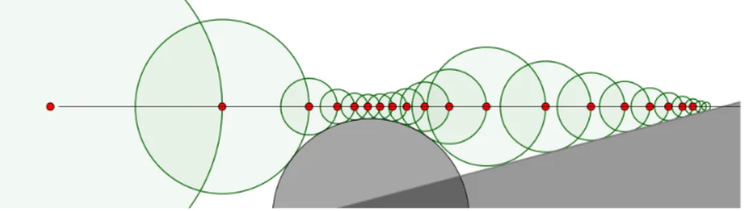
Previous work The algorithm for rendering SDFs known as sphere-tracing was first investigated by Hart in [5] (1994). It is an iterative ray-tracing algorithm, illustrated in Figure 1. This algorithm has been commonly used for the past two decades for rendering SDFs, most notably fractals [3, 4, 7, 9].

Figure 1: Illustration of the sphere-tracing algorithm in 2D.

At every point (red dot) along the ray, the distance to the surface is estimated, in this case, to the union of a half-plane and a circle. This distance defines a sphere (green circles) in which there are no intersections between the ray and the surface. Thus, sphere-tracing travels this distance

along the ray to get the next estimate of the intersection point.

Following a short overview of singed distance functions, we introduce an algorithm for algebraic surface visualization. Approximating the surface normal is common problem, for witch a novel method is presented in Section 5.

2. Signed Distance Functions

In this section, definitions and notations are introduced for future reference. Defi- nition 2.2 is from Hart’s original work in [5].

Definition 2.1(Distance to set). Let(X, d)be a metric space,x∈X, andA⊂X.

Then let d(x, A) := infa∈Ad(x, a) (whereinf∅:= +∞).

Definition 2.2 ((Signed) Distance Function). The f : Rⁿ → R function is an exact (singed) distance function, or (S)DF, if for anyppp∈Rⁿ:

1CSG, Constructive Solid Geometry: A tree-like representation of the scene using primitive objects as leaves, set operations as nodes, and transformations as edges. [2]

6 Cs. Bálint, G. Valasek

(9)

f(ppp) =d ppp, f⁻¹(0)

or f(ppp) =

(d(ppp,bound(D)) if ppp∈D

−d(ppp,bound(D)) if ppp6∈D

!

. (2.1) Where bound(D) =D\int(D)denotes the boundary of a set.

Definition 2.3 (Distance Function Estimate). The f : Rⁿ → R function is a (signed) distance function estimation if and only if there exists a q:Rⁿ →[1, K) bounded (K∈R) function, such thatf·q is a (singed) distance function.

Remark 2.4. Besides the SDF being an upper bound to the estimate, Definition 2.3 provides a lower bound for the estimate, so sphere-tracing algorithms still converge.

The following theorem by Hart [5] describes how SDFs representing objects can be combined to create more complex geometries using CSG-like constructions.

Figure 2a shows an application of the polynomial soft-min/max versions of set operations to various geometries.

Theorem 2.5 (Set operations). Let f, g∈Rⁿ→Rbe (S)DF. Then

(i){f ≡0} ∪ {g≡0}={min(f, g)≡0}, (ii){f ≡0} ∩ {g≡0}={max(f, g)≡0}, (iii) {f ≡ 0} \ {g ≡ 0} = {max(f,−g) ≡ 0}. Additionally, the min(f, g) and max(f, g)are (singed) distance function estimates.

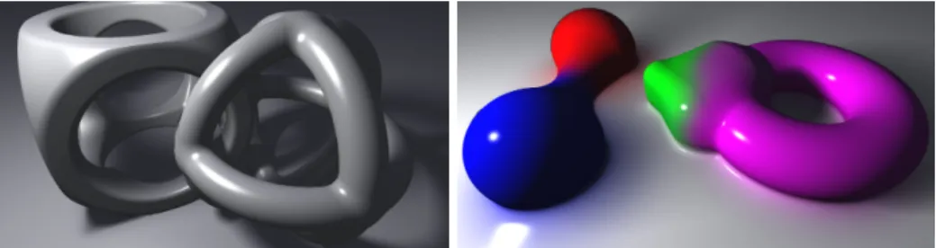
(a)Soft-min/max using 3 tori, 3 cylinders, 2

spheres, 1 cube, and 1 plane (b) Meta-surface of 2 spheres, 1 cube, 1 torus, and 1 plane

Figure 2: Demonstration of the CSG model capabilities using our rendering engine Moreover, by using different blending functions between primitive geometries one can achieve the look of different phenomena, like water [8]. Figure 2b shows meta surfaces rendered in our system.

3. Algebraic surface estimation

Let us now consider the problem of estimating SDFs to algebraic surfaces of the form f(x, y, z) =

ni

X

i=0 nj

X

j=0 nk

X

k=0

aijkxⁱy^jz^k (aijk∈R). To construct an SDF from this, we have to use the following theorem [5]

Interactive Rendering Framework for Distance Function Representations 7

(10)

Theorem 3.1. Iff∈Rⁿ→Ris a (S)DF, it is Lipschitz continuous, andLipf = 1. Therefore, for any Lipschitz continuous f function _Lip^f_f is a signed distance function estimate. Although algebraic surfaces are not Lipschitz continuous over R³, they become Lipschitz over any finite bounded subset of space. In this case, if the distance from a given point to the surface is r, the estimation would be f(ppp)/Lipf|Sr(ppp) =f(ppp)/Lip_S_r_(p_p_p)f , where Sr(ppp)is the sphere with centreppp and radiusr >0. This provides the following fixpoint-iteration

F(r, ppp) = f(ppp)

Lip_S_r_(p_p_p)f =r. (3.1) IteratingFon its first argument,r, results in an estimation of the distance function.

Usually, we have to calculate the distance in a certain direction, for example along a ray. Letsss(t) :=ppp+t·vvv. We must calculate the Lipschitz constant of the following on a given Sr(ppp)set.

f(sss(t)) =

ni

X

i=0 nj

X

j=0 nk

X

k=0

aijk(px+tvx)ⁱ(py+tvy)^j(pz+tvz)^k (3.2) The substitution method for calculatingLip_[₋_r,r]f◦sssof (3.2) is treating this expression as a f ◦sss ∈ R[t, px, py, pz, vx, vy, vz] seven variable polynomial. Mul- tiplying out, then ordering the terms, we get N ≤ ni+nj+nk + 1 number of monomials in t. LetPn(ppp, vvv)·tⁿ denote thenth monomial.

Therefore, Lip

t∈[−r,r]

(Pn(ppp, vvv)·tⁿ)≤n·rⁿ⁻¹|Pn(ppp, vvv)|is the estimate of the Lips- chitz constant of thenth monomial², where ris from (3.1), and the sum of these is the upper-estimate of the Lipschitz constant off.

The problem with this approach is that in practice, we have to be able to make symbolic calculations within the engine and generate GPU code based on the algebraic surface given.

4. Taylor-series method

Our method is based on the fact that a Taylor expansion of a polynomial is itself.

To calculate Pn(ppp, vvv) first we note that Pn = _n!¹(f ◦s)⁽ⁿ⁾(0). Now, let us find an efficient way to compute the nth derivative off ◦sss. Let

gijk(t) := (px+tvx)ⁱ(py+tvy)^j(pz+tvz)^k (t∈[−r, r]), (4.1) so Pn=

ni

X

i=0 nj

X

j=0 nk

X

k=0

aijk

g⁽ⁿ⁾_ijk(0)

n! . Lethijk(t) := ivx

px+tvx

+ jvy

py+tvy

+ kvz

pz+tvz. Note thatg⁰_ijk=gijk·hijk, sog⁽ⁿ⁺¹⁾_ijk =

Xn

m=0

n m

g_ijk^(m)h^(n−m)_ijk , where

2On estimating Lipschitz constants: [1]

(11)

h⁽ⁿ⁾_ijk(t) = (−1)ⁿ·n!

"

i px

vx

+t −n−1

+j py

vy

+t −n−1

+k pz

vz

+t −n−1#

. (4.2)

Thus,h⁽ⁿ⁾_ijk, g⁽ⁿ⁾_ijk, andPn can all be computed, and so is the following approximation:

Lip

[−r,r]

(f◦sss) = Lip

t∈[−r,r]

ni+nj+nk

X

n=0

Pn·tⁿ

!

≤ XN

n=1

n·rⁿ⁻¹|Pn|. (4.3) Finally, repeating the (3.1) iteration gives us the distance estimate.

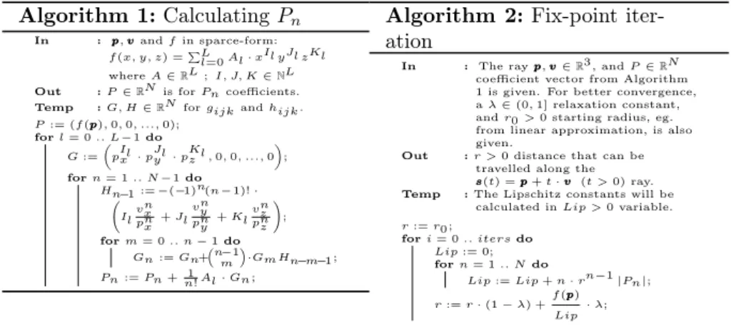
Algorithm 1:CalculatingPn

In : ppp, vvvandfin sparce-form:

f(x, y, z) =PL

l=0Al·xIl yJl zKl whereA∈RL;I, J, K∈NL Out :P∈RNis forPncoefficients.

Temp :G, H∈RNforgijkandhijk. P:= (f(ppp),0,0, ...,0);

forl= 0.. L−1do G:=

pIlx ·pJly ·pKlz ,0,0, ...,0

; forn= 1.. N−1do

Hn−1 :=−(−1)n(n−1)!· Ilvnx

pnx +Jlvny pny +Klvnz

pnz

!

; form= 0.. n−1do

Gn:=Gn+n−1 m

·GmHn−m−1;

Pn:=Pn+ 1n!Al·Gn;

Algorithm 2:Fix-point iteration

In : The rayppp, vvv∈R3, andP∈RN coefficient vector from Algorithm 1 is given. For better convergence, aλ∈(0,1]relaxation constant, andr0>0starting radius, eg.

from linear approximation, is also given.

Out :r >0distance that can be travelled along the s

s

s(t) =ppp+t·vvv (t >0)ray.

Temp :The Lipschitz constants will be calculated inLip >0variable.

r:=r0;

fori= 0.. itersdo Lip:= 0;

forn= 1.. Ndo

Lip:=Lip+n·rn−1|Pn|;

r:=r·(1−λ) +f(ppp) Lip ·λ;

Figure 3: Novel algorithms for algebraic surface visualization.

First, using equations (4.1)–(4.3), thePncoefficients of the Taylor expansion off◦sssare calculated.

Second, the fix-point iteration in (3.1) is used to find the right step size for the sphere-tracing algorithm.

Implementing this approach is easier as it does not require symbolic expres- sions and complex code generation, see the algorithms on Figure 3. Figure 4 sum- marises our results. The algorithm can be stopped at any derivative thus achieving quadratic complexity in the number of derivatives and linear in the number of terms.

Figure 4: Comparison of SDF estimations with capped amount of steps along a ray.

The algebraic surfacefK1,K2(x, y, z) = (x²+y²+z²)(K1x²+K2y²)−2z(x²+y²) = 0has a singular line that makes it hard to visualize from this angle. The Taylor method converges closer to the surface in less steps in about the same time as the traditional linear and quadratic SDF approximations. The

light-blue means it only takes one step, and in the red region it takes 70.

(12)

5. Normal estimation

The surface normal atppp∈ {f ≡0}is defined as the unit vectornormnormnorm(ppp) = _k∇^∇f(p_f(p_p_p)^p^p)_k₂, for any surface defined by the differentiable implicit functionf ∈R³→R.

In this section, we focus on calculating the normal numerically. The one-sided (forward or backward) difference method gives an error ofO()for the derivative.

A more accurate method is the symmetric difference:

∇f(x, y, z) = 1 2·





f(x+, y, z)−f(x−, y, z) f(x, y+, z)−f(x, y−, z) f(x, y, z+)−f(x, y, z−)



+O ²

. (5.1)

The idea of our approach is to take the following vectors (or stencil) vvv1:= [+1,0,0]^>, vvv3:= [0,+1,0]^>, vvv5:= [0,0,+1]^>, vvv2:= [−1,0,0]^>, vvv4:= [0,−1,0]^>, vvv6:= [0,0,−1]^>, then (5.1) is equivalent to∇f(ppp) = ₂¹ P6

i=1f(ppp+·vvvi)·vvvi, thus we define normnormnorm(ppp) = 1

Z X6

i=1

f(ppp+·vvvi)·vvvi . (5.2) where Z ∈ R is the normalising constant. This means that the samples of the function are taken at the vertices of an octahedron.

(a)Error in relation to. Line breaks when the angle between the analytic and the numeric estimation is zero.

mean median one-sided 119 562

tetrah. 113 843

octah. 1.0 1.0

cube 0.6 0.7

icosah. 0.5 0.1 dodecah. 0.5 0.1

std max

one-sided 382 306 tetrah. 265 313

octah. 1.0 1.0

cube 0.5 0.6

icosah. 0.4 0.3 dodecah. 0.4 0.3 (b) Relative error to symmet-

ric difference for= 0.01

Figure 5: Error of normal estimators measured in cosine distance³.

Our tetrahedron kernel performs slightly better than the one-sided approach and results in a marginally lower mean error with lower variance. Cube, icosahedron and dodecahedron kernels also slightly out-

performed the symmetric difference, but they also take considerably more samples.

According to our measurements, an optimal stencil vector set would consist of equal length vectors that fill the space evenly, so the best kernels in these cases

3cosine_distance(a, b) = 1−cosine_similarity(a, b) = 1−cos(θ) = 1−_k_a_k^a·b₂_·k_b_k₂

(13)

consisted of vertices of platonic solids. Taking every second vertex of a cube gives us the fastest kernel, the tetrahedron:

vvv1:= [+1,+1,+1]^>, vvv2:= [+1,−1,−1]^>, vvv3:= [−1,+1,−1]^>, vvv4:= [−1,−1,+1]^>. This is as fast as the first-order divided difference, but it gave empirically better results as shown on Figure 5. Other platonic solids were also investigated.

Potentially, even higher accuracy can be achieved by sampling surface of the unit sphere with a sequence of low discrepancy, like a Halton sequence. However, this is usually not needed, because the length of the SDF estimate’s gradient is usually close to one. Moreover, the normal is needed for calculating lighting effects, and small errors are not visible.

The implementation supports multiple normal calculation algorithms. The tetrahedron kernel proved to be faster than the first-order divided difference one.

Symmetric or octahedron kernels introduced barely visible differences in quality along hard edges.

6. Implementation

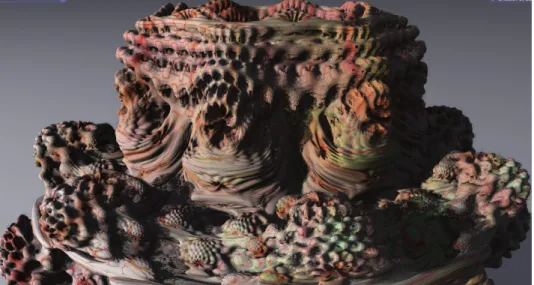
Figure 6: Mandelbulb fractal displayed with our rendering engine.

Maximum quality was reached after 156.2ms render time. Shadows were at maximum quality after 436.2ms. GPU utilisation was 97-99%. GPU: NVidia 640M (480 GFLOPS).

The rendering engine supports operating in a progressive mode, which means when the camera is not moving, the image quality continues to increase. Therefore, the engine is optimised for static scenes. The C++ and OpenGL implementation is highly efficient achieving near 100% GPU utilisation and provides several features.

Firstly, swapping algorithms between passes was a free operation due to the OpenGL subroutines running on the GPU. This and the algorithms inter-compa- Interactive Rendering Framework for Distance Function Representations 11

(14)

tibility can be used for a short statistical training to determine the best schedule of algorithms for a given scene.

Secondly, a CSG model creator was also implemented. The user can either write the program computing the SDF directly or build the CSG tree from primitives and other program codes both using a built-in graphical interface.

Finally, the shader programs, including subroutines, were generated on-the- fly, thus the code for the scene geometry is embedded into the code running on the GPU. This greatly reduced both the distance function evaluation times and memory consumption.

7. Summary

This paper presented a direct signed distance function visualisation framework and its application to rendering algebraic surfaces.

We proposed a local signed distance function estimation method to such surfaces and investigated the precision of various surface normal estimation heuristics.

We benchmarked the performance of the system by rendering complex scenes in- corporating CSG elements, meta-surfaces, and the Mandelbulb fractal.

The framework proved to be highly efficient. In addition, it is highly modular, and outperformed current fractal-viewers [3, 4, 7, 9] in both quality and speed.

References

[1] Kenneth Eriksson, Donald Estep, and Claes Johnson. Applied Mathemat- ics: Body and Soul. Number 978-3-540-00890-3. Springer-Verlag Berlin Heidelberg, 1 edition, 2004. Volume 1: Derivatives and Geometry in IR3.

[2] Gerald Farin.Curves and Surfaces for Computer Aided Geometric Design (3rd Ed.):

A Practical Guide. Academic Press Professional, Inc., San Diego, CA, USA, 1993.

[3] Paul Geisler, Daniel White, Paul Nylander, Tom Lowe, David Makin, Buddhi, Joy Leys, Knighty, and Jan Kadlec. Online fractal viewer: FractalLab.

http://hirnsohle.de/test/fractalLab/, 2010.

[4] Matthew Haggett. Mandelbulb 3D (MB3D) fractal rendering software. http://

mandelbulb.com/2014/mandelbulb-3d-mb3d-fractal-rendering-software/, 2014.

[5] John C. Hart. Sphere tracing: A geometric method for the antialiased ray tracing of implicit surfaces.The Visual Computer, 12:527–545, 1994.

[6] Benjamin Keinert, Henry Schäfer, Johann Korndörfer, Urs Ganse, and Marc Stamminger. Enhanced Sphere Tracing. In Andrea Giachetti, editor, Smart Tools and Apps for Graphics - Eurographics Italian Chapter Conference. The Euro- graphics Association, 2014.

[7] Krzysztof Marczak. Mandelbuilder - 3D fractal explorer.

http://www.mandelbulber.com/, 2010.

[8] László Szécsi and Dávid Illés. Real-time metaball ray casting with fragment lists.

In Carlos Andújar and Enrico Puppo, editors, Eurographics (Short Papers), pages 93–96. Eurographics Association, 2012.

(15)

[9] Íñigo Quílez. Mandelbulb.

http://www.iquilezles.org/www/articles/mandelbulb/mandelbulb.htm, 2009. (Mandelbulb in real time).

(16)

(17)

Scale-free property of the weights in a random graph model ^∗

István Fazekas, Attila Perecsényi

Faculty of Informatics, University of Debrecen fazekas.istvan@inf.unideb.hu perecsenyi.attila@inf.unideb.hu

Abstract

A new modification of theN interaction model [5], which based on the 3-interactions model of Backhausz-Móri [1]. This is a growing model, what evolves by weights. In every step N verticies will interact by form a star graph. We can choose vertices uniformly or according to their weights (preferential attachment). Our aim is to show asymptotic power-law distributions of the weights. The proofs are based on discrete time martingale methods.

Numerical result is also presented.

Keywords:random graph, network, scale-free, power-law MSC:05C80, 60G42.

1. Introduction

Barabási and Albert [2] gave an explanation for the frequently observed phenomenon that many real-life networks are scale free, i.e., they have power-law degree distribution. To describe real-life networks such as the WWW, social and biological networks, they introduced a random graph model. They defined an evolv- ing graph using the preferential attachment rule, what leads to scale-free graphs.

Preferential attachment rule in a random graph model means, that when a new vertex is born, then the probability that the new vertex will be connected to an old vertex is proportional to the degree of the old vertex.

∗Attila Perecsényi was supported through the New National Excellence Program of the Min- istry of Human Capacities

Annales Mathematicae et Informaticae 48(2018) pp. 15–22

15

(18)

In [4] a new network evolution model was introduced. In this paper, we shall study the same model. Consider an increasing sequence of weighted undirected graphs. The evolution of the graphs is based on creations of N-star subgraphs.

Throughout the paper we call a graphN-star graph ifN vertices form a star, that is it has one central vertex, what is connected withN−1 peripheral vertices. We start at time 0, and the initial graph is an N-star graph. This graph and all of its(N−1)-star subgraphs and all vertices have initial weights1. Now we increase the size of the graph as follows. At each step N vertices interact with each other.

It means that, we draw all non-existing edges between the peripheral vertices and the center vertex, so that, the vertices will form an N-star graph and the weights are increased by1. The non-existing elements of the graph have weight 0.

We have two options in every step. On the one hand, with probability p, we add a new vertex, and it interacts with N−1 old vertices. On the other hand, with probability1−p, we do not add any new vertex, butN old vertices interact.

Here 0< p≤1 is fixed.

When a new vertex is born, we have two possibilities again. With probability r, we choose an (N−1)-star graph according to to their weights (i.e. preferential attachment), and the new vertex is connected to its central vertex. Here preferential attachment means that the probability that we choose an (N−1)-star subgraph is proportional to its weight. With probability1−r, we chooseN−1 old vertices uniformly at random and they will form an N-star graph with the new vertex, so that, the new vertex will be the center. Here uniform choice means that all subsets of vertices with cardinalityN−1, have the same chance. Here0≤r≤1is fixed.

In the other case, when we do not add any new vertex, we have two opportunities again. On the one hand, with probabilityq, we choose an oldN-star graph according to their weights (i.e. preferential attachment). That is the chance of an N-star subgraph is proportional to its weight. Then we increase the weights inside theN-star subgraph chosen. On the other hand, with probability1−q, we choose uniformly N old vertices, and they form anN-star graph, so that, we choose the center out of the chosenN vertices uniformly. Here0≤q≤1 is fixed.

In [4] power law distribution of the weights of the vertices was shown. In this paper Theorem 2.1 shows that the weights of the N-stars have power law distribution. In the proof we use the Doob-Meyer decomposition and the method of [3].

2. Power law distribution of the weights of N-stars

Let S(n, w) denote the number of N-stars with weight w, and let Sn denote the number of allN-stars afternsteps. Furthermore,Vndenotes the number of vertices after nsteps.

Theorem 2.1. Let 0< p <1 and0< q. For all w= 1,2, . . . we have S(n, w)

Sn →sw (2.1)

16 I. Fazekas, A. Perecsényi

(19)

almost surely as n → ∞, where sw, w = 1,2, . . . are positive numbers satisfying the recurrence relation

s1= 1

h+ 1, sw=h(w−1)

hw+ 1 s_w−1, ifw >1, (2.2) whereh= (1−p)q. Moreover,

sw∼Cw⁻(¹⁺h¹) (2.3)

asw→ ∞, withC= ¹_hΓ 1 + ¹_h . Proof. First we show that

S(n, w)

n →kw (2.4)

almost surely asn→ ∞for any fixedw. Herekw,w= 1,2, . . . are fixed nonnegative numbers.

We compute the conditional expectation of S(n, w) with respect to Fn−1 for w≥1. LetS(n,0) = 0for alln. Forn, w≥1we have

E(S(n, w)|Fⁿ−1) =p(n, w−1)S(n−1, w−1) + (1−p(n, w))S(n−1, w)+

+δ1,w

"

p+ (1−p)(1−q) 1− Sn−1 V_n−1

N

!#

, (2.5)

where

p(n, w) = (1−p)

"

qw

n + (1−q) 1

V_n−1 N

N

#

. (2.6)

Let

c(n, w) = Yn

i=1

(1−p(n, w))⁻¹, w≥1. (2.7) It is easy to see that the above random variable isFⁿ−1 measurable. Applying the Marcinkiewicz strong law of large numbers for the number of vertices, we have

Vn=pn+ o

n^1/2+ε

(2.8) almost surely, for anyε >0.

Using (2.8) and the Taylor expansion forlog(1 +x)we obtain

logc(n, w) =− Xn

i=1

log 1−hw

i −(1−p)(1−q)

Vi−1

N

!

=hw Xn

i=1

1

i + O(1), where the error term is convergent asn→ ∞. It means

c(n, w)∼hwn^hw (2.9)

Scale-free property of the weights in a random graph model 17

(20)

almost surely as n→ ∞andhwis a positive random variable.

Let us consider the following process:

Z(n, w) =c(n, w)S(n, w) forw≥1.

Here {Z(n, w),Fⁿ, n= 1,2, . . .} is a nonnegative submartingale for any fixed w≥1. By the Doob-Meyer decomposition ofZ(n, w), we can write

Z(n, w) =M(n, w) +A(n, w)

whereM(n, w)is a martingale andA(n, w)is a predictable increasing process. The general form ofA(n, w)is the following:

A(n, w) =EZ(1, w) + Xn

i=2

[E(Z(i, w)|Fi−1)−Z(i−1, w)]. (2.10) Now from (2.5) and (2.10), we have

A(n, w) =EZ(1, w) + Xn

i=2

c(i, w)

"

p(i, w−1)S(i−1, w−1)+

+δ1,w p+ (1−p)(1−q) 1− S_i−1

Vi−1

N

!!#

. (2.11)

Let B(n, w) be the sum of the conditional variances of Z(n, w). In the following we give an upper bound for B(n, w):

B(n, w) = Xn

i=2

D²(Z(i, w)|Fi−1) = Xn

i=2

E{(Z(i, w)−E(Z(i, w)|Fi−1))²|Fi−1}=

= Xn

i=2

c(i, w)²E{(S(i, w)−E(S(i, w)|Fi−1))²|Fi−1} ≤

≤ Xn

i=2

c(i, w)²E{(S(i, w)−S(i−1, w))²|Fⁱ−1} ≤

≤ Xn

i=2

c(i, w)²= O n^2hw+1

. (2.12)

Above we used that c(n, w) is Fⁱ−1 measurable, (2.5) and the fact that, at each step only oneN-star is involved in interaction.

We use induction onw. Let us consider the case when w= 1. From (2.9) and (2.11), we have

A(n,1) =EZ(1,1) + Xn

i=2

c(i,1)

"

p+ (1−p)(1−q) 1− S_i−1

Vi−1

N

!#

∼

(21)

∼ Xn

i=2

h1n^h

p+ (1−p)(1−q)

1−S_i−1 i^N

∼h1

n^h+1(1−h)

h+ 1 (2.13)

as n→ ∞. Using (2.12), we have

B(n,1) = O n^2h+1 , so

B(n,1)¹²logB(n,1) = O (A(n,1)).

The conditions of Proposition VII-2-4 of [6] is fulfilled, so we have

Z(n,1)∼A(n,1) (2.14)

almost surely on the event {A(n,1)→ ∞} as n→ ∞. So from (2.9), (2.13) and (2.14), we obtain

S(n,1)

n = Z(n,1)

c(n,1)n ∼ A(n,1)

c(n,1)n ∼ h1n^h+1(1−h)

h1n^hn =1−h

1 +h =k1>0, (2.15) as n→ ∞.

Let w >1. Suppose that (2.4) is true for all weight less than w. Now from (2.8), (2.9) and (2.11), using the induction hypothesis, we obtain

A(n, w) =EZ(1, w) + Xn

i=2

(c(i, w)p(i, w−1)S(i−1, w−1))∼

∼ Xn

i=2

hwi^hwk_w−1i

hw−1

i +(1−p)(1−q) i^N

∼k_w−1hwh(w−1)n^wh+1

wh+ 1 (2.16) almost surely as n → ∞. We see that the conditions of Proposition VII-2-4 are true, so we haveZ(n, w)∼A(n, w). Therefore, from (2.9) and (2.16), we have

S(n, w)

n = Z(n, w)

c(n, w)n ∼ A(n, w)

c(n, w)n ∼ k_w−1hwh(w−1)ⁿ_wh+1^wh+1 hwn^whn =

=kw−1

h(w−1)

wh+ 1 =kw. (2.17)

Now we show that

Sn

n →B, (2.18)

almost surely as n→ ∞whereB= 1−h.

First we compute the conditional expectation ofSn with respect toFⁿ−1. We can see that the number ofN-stars increases if and only if the number ofN-stars of weight 1 increases, so we have

E{Sn|Fⁿ−1}=Sn−1+p+ (1−p)(1−q) 1− Sn−1 Vn−1

N

!

=γn−1Sn−1+B, (2.19) Scale-free property of the weights in a random graph model 19

(22)

where

γn−1= 1−(1−p)(1−q) 1

Vn−1

N

N. Let

Gn=

nY−1

i=1

(γi)⁻¹, n≥1. (2.20)

Here Gn is anFⁿ−1measurable random variable. Furthermore, let

Zn=GnSn for1≤n. (2.21)

From (2.19), we obtain

E{Zn|Fn−1}=Z_n−1+BGn. (2.22) We can see that{Zn,Fⁿ, n= 1,2, . . .} is a nonnegative submartingale. Applying again the Doob-Meyer decomposition forZn, we have

Zn =Mn+An,

whereMn is a martingale andAn is a predictable increasing process. From (2.10) and (2.22), we obtain

An=EZ1+B Xn

i=2

Gi. (2.23)

By (2.8) and applying the Taylor expansion for log(1 +x), we can give lower and upper bounds forGi, so we obtain

C1n < An< C2n, (2.24) whereC1 andC2appropriate positive constants. LetBn be the sum of the conditional variances ofZn. In the following we give an upper bound forBn:

Bn = Xn

i=2

D²(Zi|Fi−1) = Xn

i=2

E{(Zi−E(Zi|Fi−1))²|Fi−1}=

= Xn

i=2

G²_iE{(Si−E(Si|Fi−1))²|Fi−1} ≤ Xn

i=2

G²_iE{(Si−S_i−1)²|Fi−1} ≤

≤ Xn

i=2

G²_i ≤C3n, (2.25)

where C3 is a positive constant. Above we used that Gi is Fⁱ−1 measurable and the fact that, at each step, at most one N-star can be born. Using (2.25), we have Bn^1/2logBn = O(An). From (2.24), we can see that An → ∞as n→ ∞, so applying Proposition VII-2-4 of [6], we obtain

Zn∼An (2.26)

(23)

almost surely as n→ ∞.

Using (2.26) and (2.23), we have Kn

n = Zn

Gnn ∼ An

Gnn = EZ1

Gnn+B 1 Gn

1 n

Xn

i=2

Gi→B (2.27)

almost surely.

Finally, from (2.4) and (2.18), we obtain S(n, w)

Sn

=S(n, w) n

n Sn →kw

B =sw (2.28)

almost surely as n → ∞. By using (2.28) for (2.15) and (2.17), we have the recurrence of sw(cf. (2.2)). Applying several times (2.2), we obtain

sw=s1

Yw

i=2

h(i−1) hi+ 1 = 1

h

(w−1)!

Qw

j=1 j+_h¹ = 1 h

Γ(w)Γ 1 +_h¹

Γ w+ 1 + ¹_h. (2.29) SinceP∞

w=1sw= 1, the sequences1, s2, . . . is a proper discrete probability distribution.

Now applying Stirling’s formula for (2.29), we obtain the power law distribution (2.3).

3. Numerical result

In this section we present a numerical result. The4-star model was generated with parametersp= 0.5,q= 0.5andr= 0.5. We simulatedn= 10⁵ steps. To visualize the power law distribution we used log-log scale. Figure 1 shows that the weight distribution of4-stars is indeed power law distribution.

Figure 1: The weight distribution of4-stars

Scale-free property of the weights in a random graph model 21

(24)

References

[1] Backhausz Á., Móri T. F., Weights and degrees in a random graph model based on 3-interactions,Acta Math. Hungar., Vol. 143(1) (2014), 23–43.

[2] Barabási A. L., Albert R., Emergence of scaling in random networks,Science, Vol.

286 (1999), 509–512.

[3] I. Fazekas, Cs. Noszály, A. Perecsényi, Weights of Cliques in a Random Graph Model Based on Three-Interactions,Lithuanian Mathematical Journal, 55 (2015), 207- 221.

[4] I. Fazekas, Cs. Noszály, A. Perecsényi, TheN-stars network evolution model, in preparation.

[5] Fazekas, I., Porvázsnyik, B., Scale-free property for degrees and weights in an N-interactions random graph model,J. Math. Sci.Vol. 214 (2016), 69–89.

[6] Neveu, J.Discrete-parameter martingales,North-Holland, Amsterdam, 1975.

(25)

A web-based programming environment for introductory programming courses in

higher education

Győző Horváth

Eötvös Loránd University, Faculty of Informatics gyozo.horvath@inf.elte.com

Abstract

Choosing the right programming environment has a great influence on the efficiency of the educational, learning and problem solving processes. While there are many good examples for such environments for the younger generation, which involve block-based programming, gamified learning, appropriate language of the tasks and user interface design, introductory programming courses in higher education rarely take into account the role of the programming environment. In this article we have analyzed a typical problem solving process in an introductory programming course with a special focus on the programming environment. We have found that many distracting factors may make the learning process difficult.

Based on our investigation we introduce a web-based programming environment which takes into account the special needs of newcomers to the programming land. This environment tries to exclude the distracting factors and support the problem solving process in a right way. Beside our methodological considerations, the technical background of supporting traditional programming languages, such as C++, in the web browser is also presented.

Finally we make methodological recommendations how this tool can be a part of the teaching and learning process through different types of tasks and learning organizing methods.

Keywords: web, teaching, programming, development environment, higher education

MSC:97Q60, 97B40, 97U70 Annales Mathematicae et Informaticae 48(2018) pp. 23–32

23

(26)

1. Introduction

Choosing the right programming environment has a great influence on the efficiency of the educational, learning and problem solving processes. There are many good examples for such environments mainly for the younger generation, taking into account the specific needs of users of these ages. The user interface design is appropriate: nice and colourful for the youngest ones, or comes in different thematic flavours from toys, computer games or films (e.g. [1]) for teenagers. The task descriptions are usually simple and straightforward according to age of the students.

The chosen programming language is mainly block-based (like [2]) for the introductory lessons, because it hides the syntactic difficulties behind the blocks, and beginner students only have to deal with the semantic meanings of the blocks, and how to place them one after another or inside to achieve the task. And finally, task solving is often wrapped in a gamified clothes, making the learning process fun and challenging (e.g. [3]).

Introductory programming courses in higher education, however, often consid- ers novice programmer students, as if they have a lot of experience in handling complex processes, but usually this is not the case, no matter how much this would be expected. Treating them as “mature” programmers involves: using code-based programming language from the very beginning, giving them mathematical problems to solve, and using professional or professional-like integrated development environments (IDE), while students need to cope with the more essential mental model of programming. It is hard for the students without any former programming experience to take such big steps in many areas of the programming field. Curricu- lum should pay attention to gradually introduce newer and newer topics, in order to evenly distribute the cognitive load and thus make the knowledge processing much more effective by students.

Programming, however, is not just coding, it is part of a more general task, problem solving. Problem solving begins with the interpretation of the task description, continues with abstracting out and describing the data and their rela- tions contained therein (specification), then it provides a solution as a sequence of elementary steps in an abstract language (pseudo-code,algorithm), which is finally implemented in the given or chosen programming language (coding). Problem solving, however, does not end with this latter step even in a narrower scope, as we have to make sure that the program works correctly bytesting it, and the detected errors need to be corrected. For smaller programs and tasks, the problem solving may end here. Introductory courses require such programming environments that support both the basic steps and skills of problem solving and the coding phase at the same time.

In this article first we analyse a typical problem solving process in an introductory programming course with a special focus on the programming environment.

After this and based on our investigation, we look for better alternatives than using the traditional IDEs, and propose a programming environment which tries to meet the required expectations.

24 Gy. Horváth

(27)

2. Analysing traditional programming environments

In this chapter a typical problem solving process will be analysed, assuming that it takes place in an introductory programming lesson in higher education with students with different preconceptions about programming and problems solving.

In order to serve this kind of heterogeneity, the course needs to introduce every concept from the basics to build a systematic knowledge common for everyone.

Accordingly, the tasks are relatively small, even at the end of the course there are no tasks that need to be disassembled into several files.

Let us review the problem solving process from the aspect of the tools and development environments. The first step is to get to know the task. This can be done verbally, written on a board, or projected to the wall. Thetask description can be paper-based or digital. Digital material may be published on a general website or in a dedicated task library. Its format can be any of the well-known document formats (HTML, PDF, docx, etc.). Typically, the task description can be accessed in a different software environment from the one where implementation would take place.

The next two steps,specification and algorithm, are designed for planning. Plan- ning is traditionally done on paper or on a board. As a new phenomenon, however, it is increasingly common for students to write notes on their digital devices and, on the one hand, they do not have an exercise book or pen, and on the other hand, performing the above two design steps with traditional editors (e.g. text or image editors) is a much larger task than doing it manually. Thus, students are prone to skip this planning step more and more frequently. However, this article does not want to address this issue. The message of this part of problem solving is that planning considerations are implemented in a different environment or tool than coding.

The spectacular and creative part of problem solving is the implementation phase, when the plan (pseudo-code) turns into code. This step often occurs in a development environment. These specific environments are chosen because they contain all the whistles and bells needed for convenient development in the chosen programming language, as opposed to a generic code editor, where setting up a basic programming session is a time-consuming task and often the user interface does not support simple usage scenarios.

Integrated Development Environments (IDEs) are prepared with tools for editing, compiling, and running certain types of programs (such as CodeBlocks, Visual Studio, Netbeans). They are convenient to use and the default settings are often sufficient. Their big disadvantage, however, is that they are designed to write much more complex programs than an initial course needs. Usually a single file is enough for solving a simpler task, but IDEs generally think in the concept of projects with many files. Their interface is often very complicated, as they provide many func- tionalities through menus, toolbars, panels, and settings. They give much more than is needed, and this may distract the attention.

Another thing that can make the usage of any kind of desktop environment

A web-based programming environment. . . 25

(28)

problematic is the installation process. Editors should be installed in classrooms, and they need to be installed at home computers by the student. Desktop applications may have other dependencies, and they need to run on different operating systems. This complexity may lead to errors.

One of the final steps after coding is testing (followed by detecting and correcting errors), consisting of two steps: syntax and semantic checking. Syntax errors are revealed during compilation: the error list usually appears in a separate panel, and in better environments the error is indicated in the source code as well.

Semantic testing has two important parts: preparing the test cases and the executing the tests. In worse scenarios test cases are announced only verbally, but in better cases they are written to the board or to the exercise book. Testing is initially made manually: the students enter the input data manually in the command line window and monitor the response of the program. The command line usually appears in a separate window independently of the developer environment. For longer inputs, tests are written to a file, which are redirected to the standard input of the running program. Creating these test files can be done in the development environment or in another program. Redirection is often not possible in IDEs, so testing requires the opening of a command line window, which adds complexity to this step.

Development in a traditional environment is often supplemented with online judging systems (e.g. [4, 5]), which verify the code objectively. These systems usually contain only the task descriptions and the batched, automated verification services, the development is still performed in separate IDEs.

Analysing this process, several problems can be identified in the relation of programming environments and introductory courses, beginner students:

• IDEs are too general: they are general-purpose development environments, and are not intended to support specific, methodologically-based problem solving processes, which would be better for beginner students. They are only focus on the implementation part of this process.

• IDEs can not guide the student, it is left for the teacher or the students themselves.

• Other knowledges are also needed, e.g. using the command line, redirecting, uploading and downloading files.

• Considering the available number of lessons per week, teaching the different tools and the whole toolchain proportionally takes much more time than teaching the essentials of problem solving, compared to their importance.

• If students come from a gamified environment, using professional IDEs is big gap to leap through.

Looking at the number of supporting programs, the whole workflow is too complex: in order to achieve their goals, students need to focus on eight different sources of information on seven different platforms:

1. Task description (separate window)

26 Gy. Horváth

(29)

2. Design (board or exercise book) 3. Coding (IDE)

4. Compilation (IDE, separate panel) 5. Running (separate console)

6. Writing test files (separate window) 7. Testing with files (separate console)

8. Automated testing (separate web application)

Considering the heterogeneity of these introductory courses, mainly coming from the previous knowledges of students, and the complex workflow that traditional programming environments provide, some demands can be formulated against a programming environment:

• Support beginners: complex processes should be made easier or left out.

• Be specific for introductory courses: it is not needed to be prepared for solving complex tasks. Introductory courses has simple tasks. Support these and support them well.

• Support simple programs: programs consist of one file, they need to read from standard input and write to standard output.

• Support the steps of task solving process: programming environment should lead the students’ hand during the process, and should support all of the important steps of task solving process.

• Support methodology: what is important methodologically, it should be supported by the environment, if it is possible.

• Support curriculum: be flexible enough to support different introductory curriculum.

• User-friendly interface: ignore every distracting element from the user interface.

• Monitor students’ performance: support monitoring of the progression, and make room for further personalization (e.g. giving different tasks for different students based on their results).

• Stand-alone usage, practice mode: the programming environment should be used with or without the teacher’s direction.

• No installation: be platform-independent avoiding errors during installation.

3. Existing alternatives as solutions

Beside the traditional development environments there are other programming platforms that can provide an alternative solution for the problematic aspects of introductory programming courses introduced above. Every alternative environment tries to operate with a simplified user interface, where all the necessary information is available in the same program. It is common in every environment that they are web-based which provides all the features that the web platform can bring:

ubiquity, no-installation set-up for the user, easier maintenance. Of course, these environments are different according to their specific needs.

(30)

The first group of these programming environments consists of theonline learning platforms, like CodeAcademy [6] or Khan Academy [7]. They are designed to be used alone without any external guidance; they proceed forward in small steps, introducing small amount of new knowledge at one time. They are using textual descriptions or video tutorials to introduce a topic, and an online editor with automatic tests for practising. It would be hard to use them in a certain curriculum or in a lesson, and they do not support some parts of the task solving procedure, like planning, manually testing and debugging.

The members of the second group are theonline code editor environments, such as CodingGround [8], Rextester [9], jDoodle [10], or Ideone [11]. They are web- based IDEs, with single or multiple file support, and sometimes with a built-in console (CodingGround). Usually standard input can be specified, and they give back the result of the compilation and the text of the standard output. They try to be general, so they can not support many of the demands that were formulated against an introductory programming environment: there is no place to give or collect task descriptions (or at least in comments), they do not support the methodologically formed steps, they do not support testing. However, these environments are great examples, that the development of command line applications can be achieved in browsers with the help of the web-platform.

A variation of the latter group is the online programming contest platforms or code training platforms such as CodeChef [12] or Codewars [13]. They are more than the previous group in a sense that they provide task description, automated tests for checking the solution, and sometimes manual tests can be given also. But they are lack of flexibility, activity monitoring can not be fulfilled, and teachers can not give their own tasks to the system. From this point of view they operate as a combination of an online IDE and judge system.

The last group of alternative environments is consist of those online editors which try to focus on educational problems. One of those web-based platform is repl.it [14]. It started as an online IDE with a built-in console, but later it was extended with some very useful educational tools, like classroom management, creating assignments, automated tests, monitoring student activities, giving task descriptions. These features are great and comes handy in certain situations, but manual testing is missing among those features, and thus some methodology-based requirements are not fulfilled.

4. The proposed programming environment

Our proposed programming environment tries to solve those issues which come from the scattered nature of the traditional programming environments along with some methodological considerations to help beginner students in learning programming.

The first version of our in-browser programming environment [15] eliminated the distracting elements, pulled together the different type of tasks, except for the planning phase, into one user interface, where the task description, the coding area, the input and outputs of manual tests, and automatic tests took place. With these

28 Gy. Horváth

(31)

it kept the attention in one place, it supported the steps of the problem solving process, and code editing had all the features a beginner needed in a comfortable, user-friendly environment. One of the main features of the first version was that it worked in an isolated environment without internet connection (offline). But this latter feature was this environment main drawback: it narrowed the potential programming languages into JavaScript and TypeScript (or, strictly speaking, any language that can be compiled in the browser), it did not give any chance to monitor students activities, only one user test could be given.

Learning from the drawbacks of the first version, the new version of the proposed programming environment was rewritten from ground up around similar user interface design principles, but with very different operations in the background.

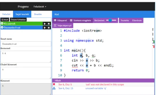
The user interface of the new environment can be seen in Figure 1. It is divided into two parts. Task description, manual and automatic tests are available in a tabbed panel on the left, while an easy-to-use and feature-rich code editor fills the right side of the browser window with the necessary buttons and informations.

The workflow is the following: students can choose among the available tasks in the drop-down menu beside the logo; can read the task description; can make the planning outside of the environment; can implement the solution in the code editor; can make multiple manual tests to determine the correctness of the solution by themselves; can verify the solution with the help of automatic test prepared by the teacher.

Figure 1: The user interface of the proposed programming environment

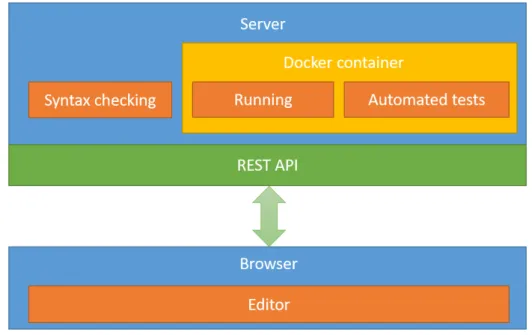
The heart of the application, the background mechanism was moved to server

(32)

side, where far more opportunities are available. The new architecture can be seen in Figure 2. Every operation that needs some language-specific feature (syntax checking, compilation, testing) sends a request to a REST API (Representational State Transfer Application Programming Interface) on the server side. Due to security reasons compilation and execution needs to be run in a sandboxed environment. The HTTP response contains the results of the requested operation, and this information is displayed on the interface.

Figure 2: The schematic architecture of the proposed programming environment

This version of the environment follows the concept of single-page applications.

The technologies that were used involves React, React-router, MobX, Monaco editor, Flexbox, Markdown on the client side, and node.js, express.js, Docker on the server.

5. Discussion and summary

The main advantage of the proposed programming environment that it keeps the problem solving process in focus (instead of the environment). It gains time both on the students’ and the teacher’s side. With different tasks and monitoring it opens up possibilities towards personalization and differentiated works. The web platform makes it possible to get rid of the installation process, to learn independently of time and place, and with sufficient automations it can offer off-class learning

30 Gy. Horváth

(33)

opportunities [16, 17].

The following type of tasks can be used in this environment:

• implementing a solution from scratch (or with minimal initial code);

• implementing one or more specific functions, the other part of the code is written already;

• correcting errors in a pre-made, but wrong program; it develops code reading.

Summarizing, the proposed web-based programming environment can help the learning processes of beginner students in an introductory programming course.

The environment is comfortable, has a non-distracting user interface, supports methodology, workflow and curriculum, and its flexible, language-agnostic architecture opens up new way towards personalisation and user monitoring. In this form it could support in-class and stand-alone usage as well.

There are many ideas for further development. User management is still missing, there should be pages where new tasks can be prepared, where task and user assignment could be achieved. User activity monitoring and personalisation would be great, and it could serve as a potential assignment platform as well. Debugging is still an issue.

References

[1] Code Studio,https://studio.code.org/[cited 2017 May 22]

[2] Scratch,https://scratch.mit.edu/[cited 2017 May 22]

[3] CodeCombat,https://codecombat.com/[cited 2017 May 22]

[4] “Bíró” judging system on the Faculty of Informatics, Eötvös University, http://biro.inf.elte.hu/[cited 2017 May 22]

[5] “Mester” judging system in Hungary,http://mester.inf.elte.hu/[cited 2017 May 22]

[6] Codecademy,https://www.codecademy.com/[cited 2017 May 22]

[7] Khan Academy,https://www.khanacademy.org/[cited 2017 May 22]

[8] CodingGround, https://www.tutorialspoint.com/codingground.htm [cited 2017 May 22]

[9] Rextester,http://rextester.com/[cited 2017 May 22]

[10] jDoodle,https://www.jdoodle.com/[cited 2017 May 22]

[11] Ideone,https://ideone.com/[cited 2017 May 22]

[12] CodeChef,https://www.codechef.com/ide[cited 2017 May 22]

[13] Codewars,http://codewars.com/[cited 2017 May 22]

[14] Repl.it,https://repl.it/[cited 2017 May 22]

[15] Horváth, Gy., Menyhárt, L.Webböngészőben futó programozási környezet meg- valósíthatósági vizsgálata,INFODIDACT 2016 Paper 3. (2016)

(34)

[16] Horváth, Gy., Menyhárt L. Oktatási környezetek vizsgálata a programozás tanításához,INFODIDACT 2014 Paper 7. (2014)

[17] Horváth, Gy., Menyhárt, L., Zsakó, L. Egy webes játék készítésének programozás-didaktikai szempontjai,INFODIDACT 2015 Paper 2. (2015)

32 Gy. Horváth

Annales Mathematicae et Informaticae (48.)

Contents

ANNALES

MATHEMATICAE ET INFORMATICAE

TOMUS 48. (2018)

COMMISSIO REDACTORIUM

HUNGARIA, EGER

ANNALES

MATHEMATICAE ET INFORMATICAE

VOLUME 48. (2018)

INSTITUTE OF MATHEMATICS AND INFORMATICS ESZTERHÁZY KÁROLY UNIVERSITY

HUNGARY, EGER

Selected papers of the

10 th International Conference

on Applied Informatics

Interactive Rendering Framework for Distance Function Representations

Csaba Bálint, Gábor Valasek

1. Introduction

2. Signed Distance Functions

3. Algebraic surface estimation

4. Taylor-series method

5. Normal estimation

6. Implementation

7. Summary

References

Scale-free property of the weights in a random graph model ∗

István Fazekas, Attila Perecsényi

1. Introduction

2. Power law distribution of the weights of N-stars

3. Numerical result

References

A web-based programming environment for introductory programming courses in

higher education

Győző Horváth

1. Introduction

2. Analysing traditional programming environments

3. Existing alternatives as solutions

4. The proposed programming environment

5. Discussion and summary

References

10 ^th International Conference

Scale-free property of the weights in a random graph model ^∗