UNIVERSITY OF PUBLIC SERVICE
UNIVERSITY OF PUBLIC
The Project is supported by the European Union and co-financed by the European Social Fund (code: EFOP-3.4.3-16-2016-00003, project title: Developing the quality of strategic educational competences in higher education, adapting to changed economic and environmental conditions and improving the accessibility of training elements).
INTRODUCTION TO
ENVIRONMENTAL DECISION SUPPORT SYSTEMS
MARK HONTI
2018
INTRODUCTION TO
ENVIRONMENTAL DECISION SUPPORT SYSTEMS
Mark Honti
2018
Table of contents
Foreword ... 3
CHAPTER I. What is a decision support system? ... 5
I.1.Environmental DSS in practice ... 10
CHAPTER II. The process of environmental decision-making ... 12
CHAPTER III. Environmental models and their uncertanity ... 16
III.1.Environmental systems and models ... 16
III.2.Model development and application ... 19
III.3.Uncertanity of models ... 21
III.4.Mathematical treatment of uncertanity... 23
III.5.Interpretation of probabilities ... 24
III.6.Main types of models ... 26
CHAPTER IV. Bayesian networks... 30
IV.1.Why use BNs in decision support? ... 36
CHAPTER V. Decision analytics ... 37
V.1.MCDA and the MAVT/MAUT approach to it ... 37
V.2.Steps of a MAVT/MAUT analysis ... 39
V.3.Why MAVT/MAUT? ... 42
V.4.Alternatives to the MAVT/MAUT approach ... 42
CHAPTER VI. Lake Balaton case study ... 45
VI.1.Background ... 45
VI.2.Decision-analytic demo of water level regulation ... 47
VI.3.Definition of the decision making context ... 47
VI.4.Structuring objectives and quantifying preferences ... 48
VI.5.Value functions ... 51
VI.6.Deficit analysis ... 52
VI.7.Predict consequences of management alternatives ... 55
VI.8.Evaluate the consequences of management alternatives ... 56
VI.9.Developing a compromise alternative ... 63
REFERENCES ... 70
FOREWORD
The ever-growing complexity of multi-layered political, administrative or economic decision-making concerning the management, use and protection of natural resources calls for enhanced decision-support tools. This applies particularly to freshwater systems where the interaction among multiple pressures, drivers and actors creates uncertainties for decison- makers with potentially long-term ramifications on the sustainablilty of aquatic resources.
The prevailing management paradigm for freshwater systems is integrated water resources management (IWRM)1. IWRM emphasises the manifold aspects of water resources management and requires that the complex natural, economical and social unit of river basins become the basis of management. This implies that decision-making should be able to handle such complex systems and the attached plethora of actors. The tremendous progress in recent years in data collection and computer-based modelling capacities decision analytics, offers tools for this – collectively referred to as decision support systems – for the enhancement of strategic policy-making.
This course material provides an introduction to the principles of environmental decision support systems to a technically non-expert audience. To that end, the following basic questions will be analysed and answered:
What is a decision support system (DSS)? What distinguishes a DSS from technical information systems, such as geographical information systems, or from models?
What can be expected from a DSS?
What cannot be expected from a DSS?
The course material will be structured as follows. First, the two main components of a DSS, i.e. predictive mathematical models and decision analytics are introduced. An overview on the main types of predictive mathematical models is provided, emphasising the unavoidable and critically important uncertainty and its types. As a special example of stochastic models, Bayesian probability networks are described in detail, for being simplified yet integrative tools for an easy comprehensive approach on environmental systems. In the decision analytical part, multi-attribute value theory (MAVT) is presented as the optimal framework for environmental decision support2, that can assist making rational decisions in the presence of uncertainty and conflicting objectives. The application of MAVT on a real, multi- stakeholder environmental problem is demonstrated in a case study (water level regulation of a touristically and ecologically important lake).
1 GWP (Global Water Partnership), 2000. Integrated Water Resources Management. Global Water Partnership,
Technical Advisory Committee, Technical Background Paper No. 5, url:
https://www.gwp.org/globalassets/global/toolbox/publications/background-papers/04-integrated-water-resources- management-2000-english.pdf (accessed at: 20.06.2018)
2 Reichert, P., Simone D. Langhans, Judit Lienert, Nele Schuwirth, 2015. The conceptual foundation of environmental decision support, Journal of Environmental Management, 154: 316-332. doi:
10.1016/j.jenvman.2015.01.053.
What will you not know?
Build a DSS.
Buid a non-trivial environmental model.
What will you know?
Understand the concept and limitations of DSSs.
Recognize cases when an environmental DSS could be beneficial.
Understand that uncertainty inherently belongs to environmental decisions.
Understand and critically assess the outputs of a DSS or communications from operators of a DSS.
Course prerequisites
Basic knowledge of mathematics and statistics Basic knowledge of logical operations
Having heard of computer models and information systems, such as Geographical Information Systems
CHAPTER I
WHAT IS A DECISION SUPPORT SYSTEM?
A formal decision problem is a situation in which a decision-maker has to select a single alternative from a finite set of possible actions3. Such problems are found everywhere in many different forms from administrative and organizational decisions to everyday life of people.
In a broad sense, a decision support system (DSS) is:
“an information system that supports business or organizational decision-making activities. (…) Decision support systems can be either fully computerized or human- powered, or a combination of both.” 4
A more precise definition is so difficult to give, that despite the 50 year old history of DSS, a consensus is still lacking. At present, systems attributed to be DSSs are ranging from simple forecasting methods to complex systems that evaluate and even propose certain decisions.5 Supporting decision-making with rational arguments based on mathematical – or in a broader sense: scientific – arguments has a long history, mainly driven by the military and optimisation of factory production. Operational research is the umbrella-term for applied mathematical methods that can solve (parts of) certain decision-making problems.
Operational research (OR) includes applications of various mathematical optimization and statistical algorithms, queueing theory, statistical process models, etc. In a broader sense, any applied mathematical exercise that targets the forecasting of a response from a managed system or the optimisation of a managed system can be considered as operational research.
As Wikipedia summarises6:
“Operational research (…) encompasses a wide range of problem-solving techniques and methods applied in the pursuit of improved decision-making and efficiency (...).
Nearly all of these techniques involve the construction of mathematical models that attempt to describe the system.”
Note, that OR is a set of techniques, it does not readily provide decision support.
As McCown summarises7, DSS is more than a set of OR procedures, it needs to replicate what human managers do in a decision-making situation:
“Although the DSS movement had pragmatic origins in OR and management science, a few DSS workers acknowledged the strong philosophical influence of ‘‘the Carnegie School’’ (e.g. Keen, 1987; Stabell, 1987). (…) They argued that a key aspect of the ‘gap’
between theory and practice was that, as humans, managers are incapable of mentally optimising practice, since optimising assumes perfect knowledge of the states and
3 Terrientes, L. M. Del Vasto, 2015. Hierarchical outranking methods for multi-criteria decision aiding. PhD Thesis Universitat Rovira i Virgili, Spain.
4 https://en.wikipedia.org/wiki/Decision_support_system
5 https://en.wikipedia.org/wiki/Decision_support_system
6 https://en.wikipedia.org/wiki/Operations_research
7 McCown, R., 2002. Locating agricultural decision support systems in the troubled past and sociotechnical complexity of ’models for management’. Agricultural Systems 74, pages 11-25.
relationships in the environment. In real life, management behaviour amounts to a search for outcomes that are satisfactory rather than theoretically best. Although inevitably failing to satisfy the criteria for substantive rationality based on what is theoretically
‘true’ in the biophysical world, this approach results in behaviour that can be shown to be procedurally rational (Simon, 1979). This so-called ‘behavioural’ approach utilises research to understand the mental processes of decision-makers managers in order to build computer programs that can mimic and improve on these internal heuristic processes. These workers linked this approach to the radical notion that human mental process can be considered analogous to symbolic information processing of digital computers—an idea that revolutionised cognitive psychology and gave rise to the field of cognitive science and artificial intelligence and to their derivatives, expert systems and knowledge-based systems.
A message implicit in this ‘cognitive revolution’ that did not go unnoticed by DSS developers was that modern management (…) was becoming so complex that without computerised decision support systems future managers will be unable to cope. This interpretation of the workplace was reinforced by burgeoning and widely publicised studies in cognitive psychology that placed emphasis on human cognitive limitations (…) i.e. having severe biases in decision making due to multiple perceptual ‘insensitivities’,
‘misconceptions’, and ‘illusions’ (Tversky and Kahneman, 1974).”
In this sense, a DSS should perform most of the decision-making procedure in case of complex systems, such as the environment. But how would such a DSS look like? The ideal DSS would be an elegant, easy-to-use software on a computer readily accessible to a manager to provide interactive assistance in the manager’s decision process8.
This (idealised) definition of DSS stems from the idea of Little9, which concentrates on the interactions between participants of decision-making. Mathematical models in OR are meant to be used by specialist systems analysts, who would provide scientifically-based guidance to decision makers10. Thus, the traditional organisational setup for a decision-making problem would involve the data, the system analyst who would apply operational reserch methods on the data and formulate rational arguments, and the decision maker, who would consider the arguments and do the decision itself. In this setup the analyst provides decision support backed up by the results from OR.
In his seminal paper Little11 proposed the concept of DSS that circumvents the human middleman (the analyst) by developing an interface directly for the manager. Although this vision was made 50 years ago, it hasn’t been realized yet, at present environmental DSSs don’t exist in a strict sense.
8 McCown (2002)
9 Little, J.D.C., 1970. Models and managers: the concept of a decision calculus. Management Science 16, pages B466– B485
10 McCown (2002)
11 Little (1970)
The biggest obstacle lies in the cornerstone of the utopian DSS: the meeting of the manager and the model. In the concept of Little the DSS meets the manager directly, so it should encompass all roles previously performed by the system analyst, which implies subject- specific intelligence, communication capabilities with the decision maker and ability to adapt when requirements change12. As McCown (2002) points out:
“A model of his operation can assist him but probably will not unless it meets certain requirements. A model that is to be used by a manager should be simple, robust, easy to control, adaptive, as complete as possible, and easy to communicate with (Little, 1970, p. B-466).”
When a management science model fails to possess any of these, it won’t be used as a DSS in Little’s sense. There have been a few applications, but the practice is an insipid picture of the promise13.
By removing the scientist middleman and giving direct data access to the decision maker, Little’s idea would simplify the organizational aspects of scientifically supported decision making. The fact that such systems have not been realized ever since, is usually considered merely as a ‘problem of implementation’14! Ironically, it was found for an agricultural DSS that success of model-based decision support improve swhen model operation is taken from the farmer to an analyst, the exact arrangement Little tried to overcome15.
McIntosh16 defines DSS based on the targeted decision contexts:
“The concept of the DSS was developed by Gorry and Morton (1971) by building on the work of Herbert Simon (1960) whose work focused on organisational decision- making. Simon (1960) distinguished three main phases of organisational decision- making (what we will term ‘decision phases’) e (i) the gathering of “intelligence” for the purpose of identifying the need for change (called “agenda setting” by Rogers, 2003); (ii) “design” or the development of alternative strategies, plans, or options for solving the problem identified during the intelligence gathering phase, and (iii) the process of evaluating alternatives and “choosing”. As described by Courtney (2001),
12 Little (1970)
13 McCown (2002)
14 McCown (2002)
15 P.S. Carberry, Z. Hochman, R.L. McCown, N.P. Dalgliesh, M.A. Foale, P.L. Poulton, J.N.G. Hargreaves, D.M.G. Hargreaves, S. Cawthray, N. Hillcoat, M.J. Robertson, The Farmscape approach to decision support:
farmers', advisers', researchers' monitoring, simulation, communication and performance evaluation, Agricultural Systems, Volume 74, Issue 1, 2002, pages 141-177.
16 McIntosh, B.S., J.C. Ascough, M. Twery, J. Chew, A. Elmahdi, D. Haase, J.J. Harou, D. Hepting, S. Cuddy, A.J. Jakeman, S. Chen, A. Kassahun, S. Lautenbach, K. Matthews, W. Merritt, N.W.T. Quinn, I. Rodriguez- Roda, S. Sieber, M. Stavenga, A. Sulis, J. Ticehurst, M. Volk, M. Wrobel, H. van Delden, S. El-Sawah, A.
Rizzoli, A. Voinov, 2011. Environmental decision support systems (EDSS) development – Challenges and best practices, Environmental Modelling & Software 26(12): 1389-1402. doi:j.envsoft.2011.09.009.
Gorry and Morton’s (1971) original innovation was to distinguish between structured, semi-structured, and unstructured decision contexts, and then to define DSS as computer-aided systems that help to deal with decision-making where at least one phase (intelligence, design or choice) was semi- or unstructured.”
A fully structured problem is unambiguous, it doesn’t leave room for considering alternatives, hence it does neither need decisions nor decision support. Thus, semi-structured or unstructured decision contexts are the key prerequisites for DSSs. According to Pidd17, decision situations can be grouped into three categories along the puzzle-problem-mess axis that describes the definitiveness of the decision problem. Structured decision contexts are puzzles, they have agreeable (or well defined) formulations and solutions. Less structured contexts are problems with agreeable formulations and arguable solutions, while messes are unstructured contexts with arguable formulations and solutions18.
The description of these categories imply that decision contexts include problem formulation and the generation and selection of solutions. A problem formulation is arguable or contested when it is generally disagreed on the very nature and the causes of the problem19. An example can be a fictional drinking water scarcity problem in a city: is the lack of sufficient amounts of drinking water a consequence of poor infrastructure, poor resource management, natural resource limitation, or oversized demand? While the above question suggests that these potential factors are mutually exclusive, in fact they can be all proper answers to some certain degree and hence the formulation is arguable or contested. When solutions are arguable or contested, different views exist on each option’s suitability to solve the problem. Translated back to the example, concurrent management options for demand reduction could be for example: increasing the price, educate clients on methods for saving water, ban certain activities (garden sprinklers, filling swimming pools, etc.), or subsidize gardens populated with plants that tolerate arid conditions20.
Following the above DSSs are the information systems meant for solving such semi- or unstructured problems. They are intended to support one or more phases of decision-making where either the decision formulation was agreeable but the solution arguable (semi- structured decision context), or the formulation and solution were both arguable (unstructured decision context)21.
17 Pidd, M., 2003. Tools for Thinking, Modelling in Management Science, Second ed. John Wiley and Sons, Chichester
18 McIntosh, B.S., Jeffrey, P., Lemon, M., Winder, N., 2005. On the design of computer-based models for integrated environmental science. Environmental Management 35, pages 741-752.
19 McIntosh et al. (2011)
20 McIntosh et al. (2011)
21 McIntosh et al. (2011)
The differences between the above two alternative definitions of a DSS highlight that it remains a theroretical challenge to identify a commonly agreed definition of a DSS22. A DSS pioneer, Keen explained:
“. . .that the intuitive validity of the mission of DSS attracted individuals from a wide range of backgrounds who saw it as a way of extending the practical application of tools, methods and objectives they believed in”23
Keen also suggested that the diverse definitions of DSS could be logically ordered on a
“Decisions+Support ––> System” spectrum that at one end emphasises the nature of the
‘Decisions’ and method of ‘Support’ and on the other end emphasises ‘System’ technology24. This construct makes explicit the sociotechnological nature of DSSs25.
Further definition attempts include more technically oriented examples too. Rizzoli and Young26 define DSS as a system of models, databases, other decision aids, all packaged in a way that decision-makers can readily use them.
Cortés defines27 an DSS as “an intelligent information system that ameliorates the time in which decisions can be made as well as the consistency and the quality of decisions, expressed in characteristic quantities of the field of application”. Besides this, environmental DSSs play an important role in helping to reduce risks resulting from the interaction of societies and the environment.
Elmahdi and McFarlane28 specifically describe an EDSS as “an intelligent analysis and information system that pulls together in a structured but easy-to-understand platform (…) the different key aspects of the problem and system: hydrological, hydraulic, environmental, socio- economic, finance-economic, institutional and political-strategic”, i.e. that EDSS should combine databases and modelling, and facilitate or be used within a participatory decision framework29.
22 Sprague Jr., R.H., 1980. A Framework for the Development of Decision Support Systems. Management Information Systems Quarterly 4, pages 1-26.
23 Keen, P.G.W., 1987. Decision support systems: the next decade. Decision Support Systems 3, pages 253–265
24 Keen (1987)
25 McCown (2002)
26 Rizzoli, A.E., Young, W.J., 1997. Delivering environmental decision support systems: software tools and techniques. Environmental Modelling and Software 12, pages 237-249.
27 Cortés, U., Sànchez-Marrè, M., Ceccaroni, L., R-Roda, I., Poch, M., 2000. Artificial intelligence and environmental decision support systems. Applied Intelligence 13 (1), pages 77-91.
28 Elmahdi, A., McFarlane, D., July 2009. A decision Support System for a Groundwater System Case Study:
Gnangara Sustainability Strategy e Western Australia MODSIM09 International Congress on Modelling and Simulation. Modeling and Simulation Society of Australia and New Zealand
29 McIntosh et al. (2011)
While definitions of a DSS can be different, they all emphasise ‘Decision Support’ to various degrees. However, DSSs, especially in the environmental contexts, have a clear secondary function as well. Besides resolving contested problems, DSS also help to increase the transparency of the decision-making process by providing an explicit description of both the problem formulation and the solution. Transparency arises because of the rational explanations provided on decisions and because of the reproducibility of the entire decision making process. It can be tested if the problem was solved in a robust way that is if slightly different problem formulation or weighing between different aspects could lead to a significantly different outcome30.
In the following, we will use a liberal definition of DSSs: all systems that contribute to rational and transparent decision making can be considered to be a DSS, given that they handle at least one non-technical aspect (that is: an economical or social attribute). The condition in the definition was added to distinguish a DSS from a model, that only considers technical aspects.
In this manner, a computer model of a catchment is not a DSS, but an extended version that helps to optimise intervention costs is a DSS.
I.1 Environmental DSS in practice
The motivation for creating environmental DSSs stems from the complexity of environmental and social problems humanity faced during the last 50 years31. From the late 20th century onwards these problems became complex, intertwined, and more and more global. Responding to such problems requires a comparably complex response from society, affecting consumption, production methods, resource management, and in general the change of attitude. Faced with such drivers for change, scientific rationality has emerged as a prominent force in environmental policy and management worldwide32. Scientific methods based on rationality provided means of approaching such complex systems and therefore became the basis for environmental policy and management worldwide. Robust scientific analysis and evidence provide support for formulating new policy objectives regarding the environment and resource utilization and this is generally accepted by the public. In conjunction with the rise of scientific rationality as a policy driver, there has been a global growth in the supply of tools and technologies to support policy assessment in various ways, accompanied by a growth in demand for decision support tools33.
30 McIntosh et al. (2011)
31 McIntosh et al. (2011)
32 McIntosh et al. (2011)
33 Nilsson, M., Jordan, A., Turnpenny, J., Hertin, J., Nykvist, B., Russel, D., 2008. The use and non-use of policy appraisal tools in public policy making: an analysis of three European countries and the European Union. Policy Science 41, 335-355
The recent extent and scale of environmental problems justify the involvement of DSS, as a technology that assists policymakers and managers in the comparative assessment of different regulation and management options.
Numerous EDSSs have been developed covering a broad focus of modelling approaches and technologies, and utilising a wide range of implicit or explicit definitions of decision support34. However, on the “Decisions+Support ––> System” scale of Keen35 most EDSS research falls on, or close to the “System” extreme. Environmental modeling is a much better developed discipline, DSS aspects only typically occupy a marginal role (that’s why we distinguish between models in a strict sense and DSSs).
Just like in other fields, EDSSs have also induced concerns36. While the technology itself is tempting, there are only few examples on real-world operating EDSSs37, and even less when such an EDSS was subject to evaluation38.
34 McIntosh et al. (2011)
35 Keen (1987)
36 McIntosh et al. (2011); Diez, E., McIntosh, B.S., 2009. A review of the factors which influence the use and usefulness of Information Systems. Environmental Modelling and Software 24 (5), 588-602.; Lautenbach, S., Berlekamp, J., Graf, N., Seppelt, R., Matthies, M., 2009. Scenario analysis and management options for sustainable river basin management: application of the Elbe-DSS. Environmental Modelling and Software 24, 26-43; Oxley, T., McIntosh, B.S., Winder, N., Mulligan, M., Engelen, G., 2004. Integrated modelling & decision support tools:
a Mediterranean example, environmental modelling and software. Special Issue on Integrated Catchment Modelling and Decision Support 19 (11), 999-1010.; Elmahdi, A., Kheireldin, K., Hamdy, A., 2006. GIS and multi-criteria evaluation: robust tools for integrated water resources management. IWRA 31 (4)
37 Cortés et al. (2000); Poch, M., Comas, J., Rodríguez-Roda, I., Sánchez-Marré, M., Cortés, U., 2004. Designing and building real environmental decision support systems. Environmental Modelling & Software 19, 857-873;
Twery, Mark J., Knopp, Peter D., Thomasma, Scott A., Michael Rauscher, H., Donald Nute, E., Walter Potter, D., Frederick, Maier, Jin, Wang, Mayukh Dass, Uchiyama, Hajime, Glende, Astrid, Hoffman, Robin E., 2005. NED- 2: a decision support system for integrated forest ecosystem management. Computers and Electronics in Agriculture 49, 24-43; Argent, R.M., Perraud, J.-M., Rahman, J.M., Grayson, R.B., Pod, G.M., 2009. A new approach to water quality modelling and environmental decision support systems. Environmental Modelling &
Software 24, 809-818.; Elmahdi et al. (2009)
38 E.g. Inman et al. (2011).
CHAPTER II
THE PROCESS OF ENVIRONMENTAL DECISION-MAKING
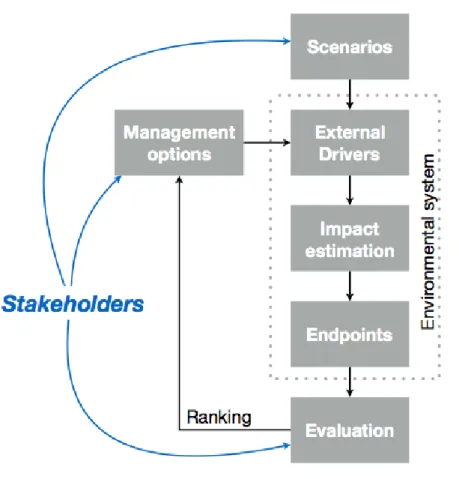
The process prior to decision making can be described by an iterative algorithm that cycles between outlining management alternatives, which are the subjects of the decision, estimating their impacts and then evaluating and ranking them (Figure 1). The actual decision is made when after some iteration cycles a certain management alternative is deemed optimal with regard to its consequences in the current decision making context. The decision about the apparently best management alternative can formally belong to three classes based on the supporting evidence:
• Accepting the management alternative (voting for its implementation), because there is enough and confident evidence about its preferable impact.
• Rejecting the management alternative (voting for not implementing it), becasue there is enough and confident evidence about its negative impact.
• Postponing the decision due to the lack of sufficient or convincing evidence for any of the previous options.
The judgement on the confidence of evidence depends on the decision making context and the principles governing the decision maker (e.g. being precautious (totally avoiding risks), or hazardous (being able to cope with certain risks)).
Figure 1. Phases of decision-support39
Figure 2. Algorithm of decision support from the environmental system perspective40.
39 Schuwirth N., Honti M., Logar I., Reichert P., Stamm C., 2018. Multi-criteria decision analysis for integrated water quality assessment and management support (manuscript)
40 Lanz, K., Eric Rahn, Rosi Siber, Christian Stamm 2013. NFP 61 – Thematische Synthese 2 im Rahmen des Nationalen Forschungsprogramms NFP 61 «Nachhaltige Wassernutzung» Bewirtschaftung der Wasserressourcen unter steigendem Nutzungsdruck. Swiss National Science Foundation. url:
http://www.snf.ch/SiteCollectionDocuments/medienmitteilungen/mm_141106_nfp61_thematische_synthese_2_
d.pdf (accessed at: 20.06.2018)
An example decision support algorithm based on the concept of value-focused thinking41 is presented here following the works of Schuwirth42. The algorithm consists of 8+1 steps (Figure 1):
1. Definition of the decision context and the scope of the decision. This includes the identification of stakeholders to be involved in the decision making process, their roles, as well as important boundary conditions.
2. Identification of fundamental objectives, which should ideally be fulfilled by the management alternatives. These should include all decision criteria considered to be important. The objectives can be structured in form of a hierarchy to facilitate the quantification of preferences.
The next steps (3. and 4.) can be carried out in different orders or even in parallel.
3. Selection of management alternatives that should be assessed.
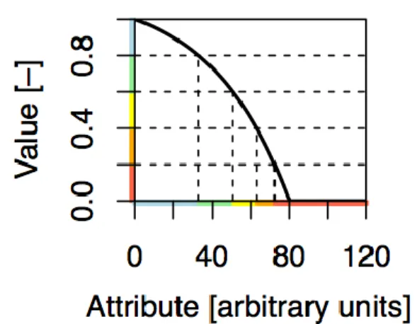
4. Quantification of preferences. Preferences can be quantified by measurable value functions43 that describe the degree of fulfillment based on quantitative measurable attributes. When multiple stakeholders are involved in the decision support process, one can elicit a value function for each person or stakeholder group.
5. Deficit analysis by applying the value function(s) to the current state. This can stimulate the planning of management alternatives44.
6. Prediction of consequences based on the current state of knowledge. While quantification of preferences reflects the subjective values of the decision maker or stakeholders, prediction of consequences must be carried out as objectively as possible.
7. If the fulfillment of the objectives monotonically increases or decreases with certain measurable attributes, a dominance analysis can rank alternatives even without knowing the full preference structure45. However, conflicting objectives are more typical for environmental decision making (for example: treatment efficency and cost). In such cases, the trade-off that stakeholders are willing to make decide which alternative is preferred.
8. Evaluation of all alternatives are evaluated based on the prediction of consequences and the quantified preferences of all stakeholders. Evaluation reveals how well the different alternatives fulfill the objectives and if there are consensus-solutions that satisfy all stakeholders or eliminate strong conflicts.
41 Keeney, R. L. 1996. Value-Focused Thinking. Harvard University Press
42 Schuwirth, N., Reichert, P., and Lienert, J., 2012. Methodological aspects of multi-criteria decision analysis for policy support: a case study on pharmaceutical removal from hospital wastewater. European Journal of Operational Research 220, pages 472–548. doi: 10.1016/j.ejor.2012.01.055
43 Dyer, J. S., and R. K. Sarin. 1979. Measurable multiattribute value functions. Operations Research 27, pages810- 822.
44 Reichert et al. (2015).
45 Eisenführ, F., Weber, M., and Langer, T., 2010. Rational Decision Making. Springer, Berlin.
9. Deficit analysis may also stimulate the creation of new alternatives, leading to an iterative procedure46.
The decision support algorithm requires two basic types of mathematical tools (Figure 2).
The prediction of consequences is basically an impact assessment of management alternatives that is usually done by models due to the complexity of environmental systems. Models are discussed in section 3. The evaluation of outcomes in a quantitative way is most often carried out by relying on Multi Criteria Decision Analysis (MCDA), due to the multitude of stakeholders and preference aspects in typical environmental problems. An implementation of MCDA via Multi-Attribute Value Theory (MAVT) is shown in the case study of section 6.
46 Hostmann, M., T. Bernauer, H.-J. Mosler, P. Reichert, and B. Truffer. 2005a. Multi-attribute value theory as a framework for conflict resolution in river rehabilitation. Journal of Multi- Criteria Decision Analysis 13:91-102.;
Hostmann, M., M. Borsuk, P. Reichert, and B. Truffer. 2005b. Stakeholder values in decision support for river rehabilitation. Archiv für Hydrobiologie. Supplementband. Large rivers 15, pages 491-505.
CHAPTER III
ENVIRONMENTAL MODELS AND THEIR UNCERTAINTY
III.1. Environmental systems and models
Environmental decision-making is complicated by the uniqueness and complexity of natural systems and the often competing needs of multiple stakeholders47. Natural systems are all different to a certain degree, that is similarities between even closely related systems are limited.
It is generally impossible to find environmental systems that are precise clones of each other, therefore one cannot apply one system as an unaffected control of another when implementing a certain management measure. Consequently, for an environmental system it is difficult to answer the following questions: “What would have happened without a certain intervention?”, and “What will happen after a certain intervention?”. Uniqueness hinders the collection of statistical evidence too. The success or the failure of a certain management method against the expectations can always be attributed to differences between the actual system and those considered as a similar reference. As a result, it is difficult to collect a homogeneous dataset of statistical evidence (contrary for example to medical treatments).
Moreover, such systems are indeed complex, especially compared to the capabilities of environmental monitoring. At the present, best available technology (and typically allocated funds) allows us to monitor up to dozens of environmental parameters with either fine spatial or temporal resolution. In contrast, even small environmental systems consist of hundreds of ecological and social actors, exhibit very high spatial heterogeneity and evolve quickly.
Consequently, environmental systems in their full complexity are beyond the bounds of our consciousness and we have to make decisions based on partial information and brutally simplified analogies on how the systems work. Therefore, uncertainty pervades all aspects of environmental decisions48.
Environmental decisions and their consequences are not repeatable in a statistical manner, that is there is no way to repeat the exact decision situation on the very same system to explore the role of pure randomness, the analysis of decision consequences is most often carried out virtually, with the help of models.
To define models, Reichert49 first defines environmental systems as: “An environmental system is a part of the natural or man-made environment, separated from the rest of the world by well- defined system boundaries” (Figure 3). In a broad sense, environmental systems range from laboratory experiments (e.g. an in vitro test of pollutant degradation, such as an OECD 308 simulation experiment) through vast areas of natural and man-made environment (e.g. river basin management planning on hundreds of thousands of km2) to the entire planet (e.g. climate change). From the perspective of decision support, systems affecting a portion of the true environment that already rises social and economic interests are of significant importance. In
47 Maier: H.R. Maier, J.C. Ascough II, M. Wattenbach, C.S. Renschler, W.B. Labiosa, J.K. Ravalico, Chapter Five Uncertainty in Environmental Decision Making: Issues, Challenges and Future Directions, Editor(s): A.J.
Jakeman, A.A. Voinov, A.E. Rizzoli, S.H. Chen, Developments in Integrated Environmental Assessment, Elsevier, Volume 3, 2008, pages 69-85.
48 Myšiak, J., Giupponi, C., Rasato, P., 2005. Towards the development of decision support system for water resource management. Environmental Modelling & Software 20, pages 203-214.
49 Reichert, P. 2012. Environmental Systems Analysis. EAWAG Dübendorf, Switzerland.
general, system boundaries should be chosen so that the system is minimal, but self-contained as much as possible at the same time.
Figure 3. The conceptual links between environmental systems and models (after Reichert 2012), here depicted on the example of a small lake and its catchment.
System boundaries should include all parts of the environment that are relevant in the investigated context, but not more to avoid unnecessary complexity. This concept is related to the impact area concept used in environmental impact assessment. A well-chosen system definition includes all parts where impact of internal mechanisms is expected to be significant (=the impact area in EIAs) and those too, from where the internal mechanisms are likely to be influenced.
Self-containment means that external influences across the system boundaries should be minimised. This does not mean that an ideal model is not exposed to any external influence factors. Environmental systems are all open to a certain degree, and hence influenced by factors more or less independent from the happenings inside the system. Even when the investigation is carried out on a global scale, external influence factors still exist. For example, during the modeling of climate change, global circulation models that describe the entire atmosphere and surface hydrology of the Earth, yet external influence factors still exist in the form of radiative forcing (e.g. the Sun’s activity) and greenhouse gas emissions from natural and man-made sources.
After defining environmental systems, Reichert50 defines models: “A theoretical construct that builds an abstract representation of a system is called a model. (…) Because of the complexity
50 Reichert (2012).
of environmental systems, such models can only be strongly simplified representations of structure and function of the underlying system.”
Detail spent on description and aggregation of certain aspects depends on the purpose of model application, on available data, on effort availability and the focus of the model study. For this reason, many models have been developed for rather similar environmental problems. For example, the prediction of river discharge from catchments as a function of rainfall and other meteorological boundary conditions have insipired dozens of structurally different models, while the basic problem is rather similar all over the temperate regions of the World. However, given that a description with full complexity was out of question for all modellers, the abovementioned factors resulted in different solutions. These factors generally mean that there is not a single, optimal, and objective model for any environmental system51. Instead, there can be several alternative descriptions of the same system in form of different models, each being adequate for addressing different set of scientific or decision support questions. These different models may differ in the detail of structure and processes, in the way they represent processes, and in the mathematical structures and formalisms used for system description.
While the definition of environmental models allows for different constructs too, in the following we focus on mathematical models. Such models use mathematical expressions represent the abstract version of the system. Building a mathematical model requires formulating knowledge and hypotheses quantitatively, and such models lead to quantitative results that can be compared for example to quantitative properties of the real system or to quantitative evaluation criteria.
Each model is constructed through the process of abstraction of observed system behaviour52. The interpretation and use of model results differs by the setup. The basic purpose of models is to estimate the system’s response as a function of external influence factors, namely unprecedented ones, otherwise historical observations could be used instead of models. When the estimated response from actual influence factors is compared to the actual response of the true system and the difference is used to fine-tune the model, the process is called calibration.
When the estimated response is still compared to the actual but the model remains untouched, the process is called validation. During validation, discrepancies between the estimated and actual responses are critically evaluated to judge if the model succeeded to grasp the essential behavioural features of the true system. When hypothetical (future) influence factors are used as the boundary conditions, the model performs true prediction.
A model is typically calibrated first (when this is possible), by adjusting its settings to match the system in question as closely as possible. Afterwards, the model needs to be validated to prove that it is a rationally acceptable abstraction of the modelled system and therefore its extrapolations to unprecedented boundary conditions can be accepted too (Figure 3). Finally, the actual utility of models is true prediction, yet the results of this phase are conditional on the results of the validation phase.
It is important to emphasise, that – similarly to any scientific theory – models cannot be proven correct. Comparing the model’s behaviour to that of the real system on data not used during
51 Reichert (2012).
52 Reichert (2012).
model creation and calibration (model validation or corroboration) can provide evidence about the representativeness of the model, but with only the following two outcomes:
• Evidence on the model replicating the real system in an acceptable way proves that the model was acceptable under the corresponding boundary conditions and internal state. In other words, this is a lack of universal counter-evidence.
• Evidence on the model failing to replicate the real system’s behaviour to an acceptable degree refutes the model universally. Such a model cannot be considered as a faithful representative of the true system.
As a consequence, a properly validated model can be considered as a model that has not been disproved yet. This maintains the future perspective for different, better models for the same purpose. As Reichert53 summarises, an ideal model properly represents the known causal relationships of the modelled system; it has a high degree of structural universality; high predictive capability; allows identifying its model parameters from measured data; and has a simple structure as long as this does not conflict with the other desired properties or the purpose of modeling.
As the definition of models suggested, models are hardly distinguishable from general scientific theories. Actually, mathematical models are formal quantitative statements about the modelled system, and as such mathematical expressions of our knowledge or belief of system functioning.
Furthermore, due to their transparent and objective definition, mathematical models can be considered as specialised languages for summarising and communicating the previously mentioned knowledge. However, the typical applied usage of models is that they are considered as rational, scientifically accepted predictors of system behaviour for unprecedented scenarios of external influence factors. As such, models are extensively used in environmental impact assessment and decision making in general.
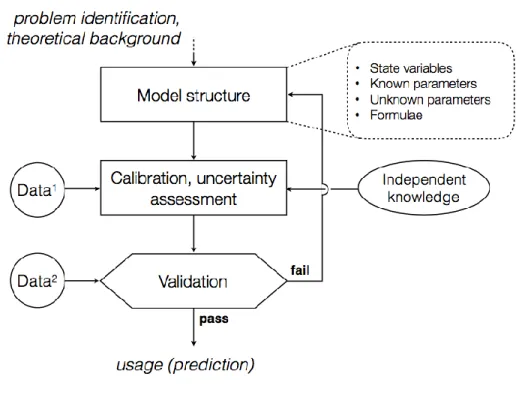
III.2. Model development and application
The application of an environmental model consists of multiple stages (Figure 4). After identifying the problem, a structure is developed based on the available theoretical background and resources. This includes the mathematical formulae, which describe the response of important quantities, the state variables in response to the external influence factors. The formulae typically contain coefficients that characterise certain inherent, time-invariable properties of the modelled system. These coefficients are called parameters. Contrary to physical models, most environmental parameters are weakly or not known due to their abstract nature and must be inferred indirectly from observations. This inference procedure is called calibration. During calibration, weakly or not known parameters are adjusted so that the model’s response matches corresponding observations about the real system as closely as possible. Calibration can utilise other, not necessarily system-specific information as well, when carried out in a Bayesian way (see section 4). Calibration alone is not sufficient to begin using the model, because fitting to certain observations does not guarantee that the characteristics of the system were fully captured. Observations that are independent from the dataset used during calibration should be used to check this in a phase called validation. During
53 Reichert (2012).
this, the calibrated model is used as if it was predicting, and the outcome is compared to the validation data. When the model’s performance is deemed sufficient, the model can be used for the dedicated purpose: prediction. In case of failure, the model needs to be revised with regard to its structure and parameter values.
Figure 4. Phases of model development.
During calibration, it has to be ensured that the model does not get overfitted. Unnecessarily complex model structures tend to increase the goodness of fit on calibration data at the price of losing generality. All environmental models have uncertainty; therefore it is not advisable to aim for a total eradication of errors during calibration. As an example, consider n observation point pairs from a linear relationship, where observations contain some random error. The proper model for such a dataset is obviously linear. However, due to the presence of errors, fit will not be perfect even after the calibration of its model parameters (the adjustment of regression constants). Increasing model complexity can obviously help. Changing the model to a higher order model will reduce calibration errors, an n-th order polynomial will even fit perfectly. The downside of this is the loss of stability in between and outside the observation points, which seriously compromises the extrapolation capabilities of the model. Overfitting can be obvious in simple cases when all observations and the entire model domain can be overviewed. In multi-dimensional, complex problems it is quite hard to detect. Therefore, the practical rule of thumb is the applied version of Occam’s razor: the best model is the simplest in terms of structure and degrees of freedom (the number of adjustable parameters) that fits the data with acceptable accuracy.
III.3. Uncertainty of models
Environmental modeling is heavily affected by uncertainty due to the uniqueness and complexity of natural systems. Environmental models often cannot reproduce the observed (past) behaviour of the modelled system within the accuracy of observations, so there are obvious errors. During predictions, there are errors too, with strong dependence on the model’s suitability for the given purpose. In most cases, prediction errors are greater than errors experienced during calibration, just like the future is more uncertain than the past (Figure 5).
The presence of uncertainty is not unique to environmental modeling. The aphorism “All models are wrong” (attibuted to statistician George E. P. Box) nicely summarises the necessary decrease of accuracy during the abstraction process of model development. Models have to be simpler than the modelled systems, and therefore they cannot reproduce the real system’s behaviour to the least detail. An improved version of the aphorism is “All models are wrong but some are useful” (G. E. P. Box), underlining that the best model for a specific purpose is still wrong, yet it provides useful and informative approximation about the modelled system.
Figure 5. True response of a system (Y, open circles), and observations about it (Yo, closed circles, containing observation errors) for the past (t < 12.5). Two models (lines) are fitted
to the observations, with the same goodness of fit. Despite having the same explaining power for the past and therefore being equally valid, predictive performance is dramatically
different in the future (shaded right half, t > 12.5), in favour of the exponential model (which still has a significant bias then). Yet, this only becomes obvious when observations
in t > 12.5 gradually become available.
Uncertainty in general is categorised into two broad types54:
• Aleatory uncertainty is real randomness. The term aleatory stems from the word ‘alea’ (lat.
‘dice’). True stochastic behaviour can be described by probability theory, which characterises
54 Reichert (2012).
events by their observed frequencies or their limits of observed frequencies upon the numerous repetitions of experiments.
• Epistemic uncertainty is uncertainty subjective to the observer or modeller due to his/her lack of knowledge (i.e. the outcome of an otherwise deterministic event becomes unpredictable for the observer as critical pieces of information are unavailable). The mathematical description of epistemic uncertainty requires a formulation that can treat knowledge or degree of belief and an algorithm that handles updating these when new pieces of empirical evidence become available. Epistemic uncertainty is inherently subjective to either individuals or groups55 (for example, scientists, modellers, or managers of a certain topic), as knowledge and beliefs cannot be universal and objective56.
Drawing the border in between the aletory and epistemic categories is a philosophical question.
One can argue that most natural (physical/chemical) systems are deterministic57 and hence all observable ‘randomness’ falls into the epistemic category. Even the outcome of throwing a dice (a purely physicl experiment) could be predicted given that all boundary and initial conditions are known precisely. On the other hand, due to the impossibility to observe everything in the finest detail, systems extremely sensible to perturbations (such as the dice to the microscopic topograpy of the table surface and to the exact path and force of the throw) are typically considered to be truly random and producing aleatory uncertainty.
The most relevant type of model uncertainty is predictive uncertainty. When a model is used for prediction (e.g. to describe the future behaviour of the modelled system, typically under different extrenal influences), the estimation of predictive uncertainty is absolutely necessary58. Components of the prediction uncertainty are usually classified as follows59:
• Aleatory uncertainty inside the system: true non-deterministic behaviour of the system.
• Epistemic uncertainty. The following sub-categories are distinguished:
• Parametric uncertainty: lack of information on the inherent, time-invariant properties of the system. In certain cases parameters may even vary in time due to improper abstractions involved in model formulation, altogether causing additional parametric uncertainty.
• Structural uncertainty: improper or incomplete formulation of the mathematical constructs.
• Uncertainty of external influence factors: improper or incomplete knowledge about the inputs and boundary conditions that the system is exposed to.
• Numerical uncertainty: imprecise solution algorithm chosen during the computer coding of the mathematical model.
55 A belief specific to a certain group of individuals is called an “inter-subjective belief”.
56 In the rational domain.
57 Outside the range of quantum effects.
58 Reichert (2012).
59 Beck: M.B. Beck, Hard or soft environmental systems?, Ecological Modelling, Volume 11, Issue 4, 1981, Pages 233-251, ISSN 0304-3800, https://doi.org/10.1016/0304-3800(81)90060-0.; Reichert (2012)
The above types describe the uncertainty of the model itself, all these components leave their imprints in the model results. It is important to emphasise, that all environmental models are affected by all these sources of uncertainty. It is only the severity of influence that may be different among models.
Whenever the model is calibrated or validated, observations about the response of the real environmental system are utilised. These are always influenced by observation uncertainty, which itself is a combination of aleatory and epistemic parts. Classical random measurement noise is aleatory, while deficiencies of the sampling design (bad choice of measurement methods, non-representative timing or spatial coverage, etc.) contribute with epistemic components to the observation uncertainty.
Due to the multitude of uncertainty sources, environmental modeling is indeed an art of living together with uncertainty. Harshly speaking, nothing is right with environmental models.
During model calibration, the results of an improperly formulated mathematical construct having badly specified parameters and propelled by error-laden external drivers are compared to observations containing errors and anyway hardly representing the behaviour of the true system. During prediction, the same model is taken to boundary conditions seldom experienced before and it is believed that the predictions still bear some meaning concerning the expected responsed of the true system. Nevertheless, models are the best rational forms of forecasting and therefore widely used. This is possible because a proper (mathematical) assessment and acknowledgement of uncertainty enables modellers to estimate the credibility of their predictions and therefore imprecise predictions can still provide a basis for rational decisions
60.
III.4. Mathematical treatment of uncertainty
Probability theory is a framework building on axioms61 designed to describe true randomness62. Relative frequencies fulfill the probability axioms. Therefore, probability theory is the obvious choice to describe aleatory uncertainty63 – no wonder, it was developed for that. An additive benefit is that probability theory is widely known and taught everywhere, and therefore its concepts are familiar to most decision-makers, which facilitates communication.
The mathematical treatment of epistemic uncertainty is less obvious. Several alternative theories exist and therefore there is no obvious choice for quantifying subjective knowledge or beliefs64. Nevertheless, conformity to certai rationality axioms can provide some hint.
Reichert65 found that there were three requirements of rationality that all independently suggested probability theory as the optimal mathematical framework for the description of subjective knowledge and beliefs:
60 Reichert, P., and Borsuk, M. E., 2005. Does high forecast uncertainty preclude effective decision support?
Environmental Modeling and Software 20 (8), 991–1001. doi:10.1016/j.envsoft.2004.10.005
61 Briefly, by Kolmogorov’s formulation: probability of an outcome is a non-negative number; the probability of at least one outcome happening from the set of all possible outcomes is 1; the probability of a sequence of mutually exclusive outcomes is the sum of their probabilities.
62 Reichert (2012).
63 Reichert (2012).
64 Reichert (2012).
65 Reichert (2012).
1. If one assumes beliefs to be rational (e.g. the person stating beliefs wants to avoid sure loss and two events having the same risks are indifferent for him/her), then probabilities must be used to describe beliefs.
2. If we request that the beliefs follow the rational rules of conditionality (a. Belief in event A not happening is a function of a belief in the contrary [event A happening]. b. Belief in events A and B happening together is a function of the beliefs of event A happening given that event B happened and the belief in event B happening.), then probabilities must be used to describe beliefs. This assumption is the Theorem of Cox (Cox, 1946), and is important for decision support because among others, management measures are boundary conditions that need to be considered when evaluating a certain outcome66. 3. Many systems exhibit some random behaviour besides being primarily deterministic.
Uncertainty about such system can be predominantly epistemic when knowledge and observations are insufficient. By increasing the body of evidence, epistemic uncertainty should gradually become equal to the aleatory uncertainty. If we require this to be a smooth transition, then the same mathematical framework must be used for both types67. However, classical probability theory needs extensions to be able to cope with subjective beliefs. The extension is called Bayesian statistics.
III.5. Interpretation of probabilities
The interpretation of probabilities in classical – so called frequentist – statistics is based on the reproducibility of random events and their outcomes. A frequentist probability is only interpreted for a truly random events – which are reproducible –, as the limit of relative frequencies of a certain outcome. The probability for a certain outcome is the proportion of these outcomes divided by the number of tries (=the number of all outcomes), as this latter increases to infinity. When a frequentist probability is estimated from limited evidence, the estimation will contain errors, the level of which depending on the number of experiments and the number of the specific outcome. Remember the case of throwing a dice: What is the probability estimate for getting a 5? From a single throw one can guess 100% or 0%, depending if the outcome was a 5 or not. While this estimate is rational, there is no evidence besides the result of the one and only throw, the uncertainty of this estimation – the confidence interval – spans the entire probability range: 0–100%. By doing more throws, the estimate converges to around 1/6 and its confidence interval gradually reduces. Yet, an immense number of tries is required to get a very precise empirical estimate of the probability and a negligible error range.
Most environmental systems show some random behaviour due to extreme sensitivity to certain initial conditions and external influence factors. It is often reasonable to describe such non- deterministic behaviour by putting stochastic elements into the model structure68. Frequentist probabilities and inference techniques (such as the likelihood method) provide a consistent framework for that, yet inference becomes seriously weak when system identification is problematic – a typical situation for environmental models. The most powerful application of
66 Reichert (2012).
67 Compare this to the fuzzy border between aleatory and epistemic uncertainties. Are there any, truly stochastic systems or just cases with insufficient knowledge?
68 Reichert (2012).
frequentist statistics in environmental modelling is the testing of hypotheses formulated as the model itself.
The Bayesian interpretation of probabilities is less restrictive than the frequentist one. This epistemic probability interpretation allows assigning probabilities to any subjective belief, not just only truly random events. By using the classical frequentist rules for conditional probability, Bayesian statistics allows a mathematical treatment of incremental learning, the reduction of epistemic uncertainty by considering newly acquired data69.
In the beginning step of an incremental learning problem one possesses some more or less uncertain knowledge or belief or expectation about the subject. This is called the a priori (or shortly: prior) knowledge and is typically uncertain due to epistemic reasons. Prior knowledge can be characterized by a Bayesian probability distribution, that assigns a probability to each possible outcome or state of the subject. The probability must be proportional to the strength of belief. During the learning step the prior knowledge is updated by incorporating information from the evidence, that is the observed state or outcome of the subject. The knowledge after the update step is called a posteriori (or posterior) knowledge and can be also characterized by a Bayesian probability distribution. The update takes place following Bayes’ law of conditional probability:
Pposterior(knowledge given evidence) = Pprior(knowledge) × L(evidence given knowledge) / P(evidence)
where P indicates Bayesian probability, and L is the so called likelihood, that specifies the probability of getting a certain evidence given the specific knowledge. Since the absolute probability for the observed evidence is independent of the knowledge, it can be left out, leaving:
Pposterior(knowledge given evidence) ~ Pprior(knowledge) × L(evidence given knowledge) where the ~ sign indicates proportionality. During the update, the following options can happen:
• When the evidence was informative
o and it was not conflicting the prior knowledge, the posterior distribution is narrower than the prior one, that is our knowledge gets more precise. In other words, the uncertainty of the prior knowledge reduces by learning, but the posterior does not refute the prior.
o but it strongly conflicts the prior knowledge, the posterior distribution is dominated by the likelihood and will be placed away from the prior. This means that the prior gets refuted by the evidence.
• When the evidence was not informative, the posterior distribution is equal to the prior that is our knowledge is the same after the update as before (a logical outcome when the evidence cannot provide any useful information).
69 Reichert (2012).