Annales Mathematicae et Informaticae (46.)

(1)

ANNALES

MATHEMATICAE ET INFORMATICAE

TOMUS 46. (2016)

COMMISSIO REDACTORIUM

Sándor Bácsó (Debrecen), Sonja Gorjanc (Zagreb), Tibor Gyimóthy (Szeged), Miklós Hoffmann (Eger), József Holovács (Eger), Tibor Juhász (Eger), László Kovács (Miskolc), László Kozma (Budapest), Kálmán Liptai (Eger), Florian Luca (Mexico), Giuseppe Mastroianni (Potenza), Ferenc Mátyás (Eger),

Ákos Pintér (Debrecen), Miklós Rontó (Miskolc), László Szalay (Sopron), János Sztrik (Debrecen), Gary Walsh (Ottawa)

HUNGARIA, EGER

(2)

ANNALES MATHEMATICAE ET INFORMATICAE International journal for mathematics and computer science

Referred by

Zentralblatt für Mathematik and

Mathematical Reviews

The journal of the Institute of Mathematics and Informatics of Eszterházy Károly University of Applied Sciences is open for scientific publications in mathematics and computer science, where the field of number theory, group theory, constructive and computer aided geometry as well as theoretical and practical aspects of programming languages receive particular emphasis. Methodological papers are also welcome. Papers submitted to the journal should be written in English. Only new and unpublished material can be accepted.

Authors are kindly asked to write the final form of their manuscript in L^ATEX. If you have any problems or questions, please write an e-mail to the managing editor Miklós Hoffmann: hofi@ektf.hu

The volumes are available athttp://ami.ektf.hu

(3)

MATHEMATICAE ET INFORMATICAE

VOLUME 46. (2016)

EDITORIAL BOARD

Sándor Bácsó (Debrecen), Sonja Gorjanc (Zagreb), Tibor Gyimóthy (Szeged), Miklós Hoffmann (Eger), József Holovács (Eger), Tibor Juhász (Eger), László Kovács (Miskolc), László Kozma (Budapest), Kálmán Liptai (Eger), Florian Luca (Mexico), Giuseppe Mastroianni (Potenza), Ferenc Mátyás (Eger),

Ákos Pintér (Debrecen), Miklós Rontó (Miskolc), László Szalay (Sopron), János Sztrik (Debrecen), Gary Walsh (Ottawa)

INSTITUTE OF MATHEMATICS AND INFORMATICS ESZTERHÁZY KÁROLY UNIVERSITY OF APPLIED SCIENCES

HUNGARY, EGER

(4)

HU ISSN 1787-6117 (Online)

A kiadásért felelős az Eszterházy Károly Egyetem rektora Megjelent a Líceum Kiadó gondozásában

Kiadóvezető: Grebely Gergely Felelős szerkesztő: Zimányi Árpád Műszaki szerkesztő: Tómács Tibor Megjelent: 2016. december Példányszám: 30

Készítette az

Eszterházy Károly Egyetem nyomdája Felelős vezető: Kérészy László

(5)

Statistics in words and partitions of a set

Walaa Asakly

Department of Mathematics, University of Haifa, Haifa, Israel walaa_asakly@hotmail.com

Submitted December 30, 2015 — Accepted September 12, 2016

Abstract

Let[k] ={1,2, . . . , k}be an alphabet overkletters. Awordωof lengthn over alphabet[k]is an element of[k]ⁿand is also called ak-ary word of length n. We say thatωcontains an`-peak, if it exists anisuch that2≤i≤n−` where ωi = ωi+1 = · · · = ω_i+`−1 and ω_i−1 < ωi and ω_i+`−1 > ωi+`. A partitionΠ of set[n]of sizek is a collection{B1, B2, . . . , Bk}of non empty disjoint subsets of[n], calledblocks, whose union equals[n]. In this paper, we find an explicit formula for the generating function for the number of words of lengthnover alphabet[k]according to the number of`-peaks in terms of Chebyshev polynomials of the second kind. As a consequence of the results obtained for words, we finally find the number of`-peaks in set partitions of [n]with exactlyk blocks.

Keywords:Set partitions, words,`-peak, Chebyshev polynomials of the second kind

MSC:05A05

1. Introduction

Words

Let [k] = {1,2, . . . , k} be an alphabet over k letters. A word ω of length n over alphabet[k]is an element of[k]ⁿ and is also called a word of lengthnonkletters or a k-ary word of length n. The number of the words of lengthnover alphabet [k] is kⁿ. Similar statistics in patterns of subwords have been widely studied in the literature (see [2]). For example, Kitaev, Mansour and Remmel [3] enumerated the number of rises (respectively, levels and falls) which are subword patterns 12,

http://ami.ektf.hu

3

(6)

(respectively,11and21) in words that have a prescribe first element. Heubach and Mansour [2] enumerated the number of words of length n over alphabet [k] that contain the subword pattern 111 and the subword pattern 112 exactly r times.

Burstein and Mansour [1] generalized the result to subword pattern of length `.

More recently, Mansour [4] enumerated the number of peaks (subword patterns 121,132or231) and valleys (subword patterns212,213or312) in words of length n over alphabet [k]. Our aim is to extend this result to patterns of arbitrary length. We say that ω contains an `-peak, if exists 2 ≤ i ≤ n−` such that ωi = ωi+1 = · · · =ω_i+`−1 and ω_i−1 < ωi and ω_i+`−1 > ωi+`. For example, the word 12⁴13⁴2 = 12222133332 in [3]¹¹ contains two 4-peaks, namely 122221 and 133332.

Set partitions

A partition Π of set[n] with exactly k blocks is a collection {B1, B2, . . . , Bk} of non empty disjoint subsets of [n] whose union is equal to [n]. We assume that blocks are listed in increasing order of their minimal elements, that is, minB1 <

minB2 < · · · < minBk. We denote the set of all partitions of [n] with exactly k blocks to be Pn,k. The number of all partitions of[n]with k blocks is S(n, k), these are the Stirling numbers of the second kind [9]. We denote the set of all partitions of [n] to bePn, namely Pn = ∪ⁿk=0Pn,k. The number of all partitions of[n]isBn=Pn

k=0Sn,k, which is then-th Bell number. Any partitionΠ can be written asπ1π2· · ·πn, wherei∈Bπi for alli, and this form is called thecanonical sequential form. For exampleΠ ={{12},{3},{4}}is a partition of[4], the canoni- cal sequential form isπ= 1123. Several authors have studied different statistics on Pn (see [4]). For instance, Mansour and Munagi [6] found the generating function for the number of partitions of[n]according to rises, descents and levels, they also computed the total number oft-rises (respectively,t-descents and t-levels), this is a increasing subword pattern of sizet(respectively, decreasing subword pattern of size t, fixed subword pattern of sizet), see [5]. A lot of attention has been given to the statistics on Pn,k (see [4]). For example, Shattuck [8] counted the rises, descents and levels in the set partition of [n] with exactly k blocks. In addition, Mansour [4] found an explicit formula for the generating functions for the number of set partition of[n]with exactlykblocks according to the statistics`-rise (respectively,`-descent and`-level). Mansour and Shattuck [7] found an explicit formula for the generating function of set partitions ofnwith exactly[k]blocks according to the number of peaks (valleys). Our aim is to extend this result for the set Pn,k

according to the number of`-peaks.

In this paper, we find the generating function of the words of length n over alphabet[k]according to the number of`-peaks. We also compute the total number of `-peaks in the words of length n over alphabet [k]. As a consequence of these results, we find the number of`-peaks in set partitions of[n]with exactlykblocks.

(7)

2. Words and partitions of a set according to multi statistics ` -peaks

LetWk(x, q1, . . . , q`)be the generating function for the number of words of length nover alphabet[k]according to the number of`-peaks, namely,

Wk(x, q1, . . . , q`) =X

n≥0

xⁿ X

ω∈[k]ⁿ

Y` i=1

qⁱ_i⁻^peak(ω).

Lemma 2.1. The generating functionWk(x, q1, . . . , q`)satisfies the recurrence relation

Wk(x, q1, . . . , q`)

= A`−xB`+W_k−1(x, q1, . . . , q`)(B`+1−A`)

(1−x)(1 +A`) +x^`+1−Wk−1(x, q1, . . . , q`) (1−x)A`+x^`+1, whereA`=P`

i=1xⁱqi andB`=¹₁⁻₋^x_x^`. Proof. It is obvious

Wk(x, q1, . . . , q`) =Wk−1(x, q1, . . . , q`) +W_k^†(x, q1, . . . , q`), (2.1) where W_k^†(x, q1, . . . , q`) is the generating function for the number of words ω of lengthnover alphabet[k]according to the number of`-peaks such thatωcontains at least one occurrence of the letterk. A wordω that contains a letter k can be decomposed as either

(1) k;

(2) kω⁰, whereω⁰ is a non empty word over [k];

(3) ω⁰⁰kⁱω⁰⁰⁰, wherekⁱ denotes a wordkk· · ·kwith exactlyiletters,ω⁰⁰ is a non empty word over[k−1]and ω⁰⁰⁰ is a non empty word over [k]which starts with a lettera6=k, for1≤i≤`;

(4) ω⁰⁰kⁱ, for1≤i≤`; or

(5) ω⁰⁰k^`+1ω⁰⁰⁰⁰, whereω⁰⁰⁰⁰is a word over[k].

The corresponding generating functions of these decomposition are (1) x;

(2) x(Wk(x, q1, . . . , q`)−1);

(3) qixⁱ(Wk−1(x, q1, . . . , q`)−1)(Wk(x, q1, . . . , q`)(1−x)−1), for1≤i≤`; (4) xⁱ(W_k−1(x, q1, . . . , q`)−1), for1≤i≤`; or

(8)

(5) x^`+1(Wk−1(x, q1, . . . , q`)−1)Wk(x, q1, . . . , q`), respectively. Hence, by (2.1), we obtain

Wk(x, q1, . . . , q`)

=Wk−1(x, q1, . . . , q`) +x+x(Wk(x, q1, . . . , q`)−1) +

X` i=1

qixⁱ(Wk−1(x, q1, . . . , q`)−1)(Wk(x, q1, . . . , q`)(1−x)−1)

+ X` i=1

xⁱ(Wk−1(x, q1, . . . , q`)−1)

+x^`+1(Wk−1(x, q1, . . . , q`)−1)Wk(x, q1, . . . , q`), which equivalent to

Wk(x, q1, . . . , q`)

= A`−xB`+W_k−1(x, q1, . . . , q`)(B`+1−A`) (1−x)(1 +A`) +x^`+1−Wk−1(x, q1, . . . , q`)

(1−x)A`+x^`+1

, (2.2)

whereA`=P`

i=1xⁱqi andB`= ^1−x_1−x^`.

We plan to find an explicit formula for the generating functionPk(x, q1, . . . , q`) for the number of partitions ofnwith exactlykblocks according to the number of

`-peaks.

Pk(x, q1, . . . , q`) =X

n≥0

xⁿ X

π∈Pn,k

Y` i=1

q^i−peak(π).

To do that we will use Lemma 2.1.

Theorem 2.2. For all k≥1, Pk(x, q1, . . . , q`)

= Yk j=1

X` i=1

xⁱ(qi(Wj(x, q1, . . . , q`)(1−x)−1) + 1) +x^`+1Wj(x, q1, . . . , q`)

! .

Proof. Any partitionπof [n]with exactlyk blocks can be decomposed either (1) πkⁱπ⁰,πkⁱ, for1≤i≤`, whereπis a set partition with exactlyk−1blocks,

π⁰ is a non empty word over alphabet[k]which starts with a lettera < k; or (2) πk^`+1π⁰⁰, whereπ⁰⁰ is a word over alphabet[k].

The corresponding generating functions are

(9)

(1)

qixⁱPk−1(x, q1, . . . , q`)(Wk(x, q1, . . . , q`)

−xWk(x, q1, . . . , q`)−1) +xⁱP_k−1(x, q1, . . . , q`), for1≤i≤`;

(2) x^`+1P_k−1(x, q1, . . . , q`)Wk(x, q1, . . . , q`),

respectively. By summing all the last terms we obtain Pk(x, q1, . . . , q`)

= X` i=1

qixⁱPk−1(x, q1, . . . , q`)(Wk(x, q1, . . . , q`)−xWk(x, q1, . . . , q`)−1)

+ X` i=1

xⁱPk−1(x, q1, . . . , q`) +x^`+1Pk−1(x, q1, . . . , q`)Wk(x, q1, . . . , q`)

=P_k−1(x, q1, . . . , q`)·

· X` i=1

xⁱ(qi(Wj(x, q1, . . . , q`)(1−x)−1) + 1) +x^`+1Wj(x, q1, . . . , q`)

! .

Thus, by induction on ktogether with the initial conditionP0(x, q) = 1, we com- plete the proof.

Example 2.3. Using the recursion given in Theorem 2.2, we may obtain the generating function for the number of partitions of[n]with exactlyk blocks,

Pk(x,1, . . . ,1) = Yk j=1

X` i=1

xⁱWj(x,1, . . . ,1)(1−x) +x^`+1Wj(x,1, . . . ,1)

= Yk j=1

x1−x^`

1−x 1

1−jx(1−x) +x^`+1 1 1−jx

=x^k Yk j=1

1 1−jx,

which is in accord with the well-known the generating function for the number of partitions of [n]with exactlyk blocks.

Example 2.4. By substituting `= 1 and q1 =qin Lemma 2.1, we get Wk(x, q) the generating function for the number of words of length nover the alphabet[k]

according to the number of peaks (peak of length one), which gives the following recursion

Wk(x, q) = x(q−1) + (1−x(q−1))Wk−1(x, q) 1−x(1−q)(1−x)−x(x+q(1−x))Wk−1(x, q).

(10)

By using the same substitution in Theorem 2.2, we obtain the recurrence relation for the generating function for the number of set partitionsPn,k according to the number of peaks (peak of length one), which gives the following recursion

Pk(x, q) =x^k Yk j=1

(1 +x(1−q)Wj(x, q) +q(Wj(x, q)−1)),

where the two above results agree with the results of Mansour and Shattuck (see [7]).

2.1. Counting `-peaks in words and partitions of a set

LetWk(x, q)be the generating function for the number of words of lengthn over alphabet[k]according to the number of`-peaks.

Wk(x, q) =X

n≥0

xⁿ



 X

ω∈[k]ⁿ

q^`⁻^peak(ω)



.

Corollary 2.5. The generating functionWk(x, q)for the number of words of length n over alphabet[k]according to the number of `-peaks is

Wk(x, q) = A+ (1−A)Wk−1(x, q)

a`−xW_k−1(x, q)a_`−1 (2.3) whereA=x^`(q−1) anda`= 1 +x^`(q−1)(1−x), which is equivalent to

Wk(x, q) = x^`(q−1)(Uk−1(t)−Uk−2(t))

Uk(t)−Uk−1(t)−(1−x^`(q−1))(Uk−1(t)−Uk−2(t)), (2.4) wheret= 1 +^x^`+1₂ (1−q) andUmis them-th Chebyshev polynomial of the second kind.

Proof. By substitutingqi= 1fori6=`, andq`=qin (2.2) we obtain (2.3). Then, by applying [Appendix D] [4] for (2.2), we obtain (2.4).

Now, our aim is to find the total number of `-peaks in all words of length n over alphabet[k].

Lemma 2.6. For all k≥1, d

dqWk(x, q)|^q=1= x^`+2 (1−kx)²

2

k 3

+ k

2

.

Proof. We compute the number of`-peaks in all the words of lengthnover alphabet [k]. By differentiating (2.3) with respect toq, we obtain

Vk(x) = d

dqWk(x, q)|^q=1

(11)

= (x^`(1−W_k−1(x,1)) +V_k−1(x))(1−xW_k−1(x,1)) (1−xWk−1(x,1))²

−Wk−1(x,1)(x^`(1−x)(1−Wk−1(x,1))−xVk−1(x)) (1−xWk−1(x,1))² , and usingWk(x,1) = ₁₋¹_kx (easy to prove by induction), we obtain

d

dqWk(x, q)|^q=1= x^`+2 (1−kx)²

2

k 3

+ k

2

, (2.5)

as claimed.

By finding the coefficient ofxⁿ in (2.5) we get the following result

Corollary 2.7. The total number of `-peaks in all the words of length n over alphabet [k] is given by

(n−1−`)k^n−2−`

2

k 3

+ k

2

.

We plan to find the explicit formula for the generating functionPk(x, q)for the number ofPn,k according to the number of`-peaks.

Pk(x, q) =X

n≥0

xⁿ



 X

π∈Pn,k

q^`⁻^peak(π)



.

Corollary 2.8. For all k≥1, the generating functionPk(x, q)is given by x^k

Yk j=1

Wj(x, q)(1 +x^`−1(x−1)) +x^`−1+qx^`−1(Wj(x, q)(1−x)−1) .

Proof. By substitutingqi= 1fori6=`, andq`=qin Theorem (2.2).

Lemma 2.9. For all k≥3, d

dqPk(x, q)|^q=1= x^{k+` k}₂

(1−x)· · ·(1−kx)+ x^k+`+2 (1−x)· · ·(1−kx)

Xk j=3

2 ^j₃ + ₂^j (1−jx) . Proof. By Corollary 2.8, we have

d

dqPk(x, q)|^q=1=Pk(x,1) Xk j=1

q→1lim

d dqLj(q)

Lj(q)

!

, (2.6)

where

Lj(q) = (Wj(x, q)(1 +x^`⁻¹(x−1)) +x^`⁻¹+qx^`⁻¹(Wj(x, q)(1−x)−1).

(12)

Note that

qlim→1

d

dqLj(q) = lim

q→1

d

dqWj(x, q) +x^`⁻¹(Wj(x, q)(1−x)−1)

= x^` (j−1)−(j−1)jx+ (2 ₃^j + ₂^j

)x²

(1−jx)² =x^` j−1

1−jx+(2 ^j₃ + ^j₂

)x² (1−jx)²

! .

Hence, by using (2.6) we obtain d

dqPk(x, q)|^q=1= x^k+`

(1−x)· · ·(1−kx) Xk j=1

j−1 +(2 ^j₃ + ^j₂

)x² (1−jx)

!

= x^{k+` k}₂

(1−x)· · ·(1−kx)+ x^k+`+2 (1−x)· · ·(1−kx)

Xk j=3

2 ₃^j + ₂^j (1−jx) , as required.

By using the facts thatPk(x,1) = P

n≥1Sn,kxⁿ and Pk

j=1(j−1)x^` =x^{` k}₂ together with Lemma 2.9 we get the following corollary. ,

Corollary 2.10. The total number of the`-peaks in all set partitionsPn,k is given

by k

2

Sn−`,k+

n−k

X

i=`+2

Sn−i,k

Xk j=3

j^i−`−2

2 j

3

+ j

2

.

2.2. Applications

By substituting`= 2 in Corollary 2.7, we obtain the following result

Corollary 2.11. The total number of the2-peaks in all the words of lengthnover alphabet [k] is given by

(n−3)kⁿ⁻⁴

2 k

3

+ k

2

. By substituting`= 2in Corollary 2.10, this leads to

Corollary 2.12. The total number of the2-peaks in all set partitionsPn,k is given

by k

2

Sn−2,k+

nX−k i=4

Sn−i,k

Xk j=3

jⁱ⁻⁴

2 j

3

+ j

2

.

By substitutingq = 0in (2.4), we obtain that the generating function for the number of words of lengthnover alphabet[k]without`-peaks is given by

Wk(x,0) = −x^`(Uk−1(t)−Uk−2(t))

Uk(t)−Uk−1(t)−(1 +x^`)(Uk−1(t)−Uk−2(t)), (2.7)

(13)

wheret= 1 +^x^`+1₂ andUmism-th Chebyshev polynomial of the second kind. By substitutingq= 0in Corollary 2.8, we get

Pk(x,0) =x^k Yk j=1

Wj(x,0)(1 +x^`⁻¹(x−1)) +x^`⁻¹

, (2.8)

by substituting (2.7) into (2.8), and using the relationUj+1(t) = 2tUj(t)−Uj−1(t), we get

Pk(x,0) =x^k Yk j=1

Uj−1(t)−(1 +x^`)Uj−2(t) (1−x)Uj−1(t)−Uj−2(t),

where t= 1 +^x^`+1₂ , which is the generating function ofPn,k without`-peaks. By using the above result with ` = 1, we obtain the same result of Mansour and Shattuck (see [7]).

Corollary 2.13. The generating function for the number of set partitions of Pn

without`-peaks is given by

1 +X

k≥1

Pk(x,0) =X

k≥0

x^k Yk j=1

Uj−1(t)−(1 +x^`)Uj−2(t) (1−x)Uj−1(t)−Uj−2(t),

wheret= 1 +^x^`+1₂ andUmis them-th Chebyshev polynomial of the second kind.

2.3. Conclusion

In the present paper, we determined the generating function for the number of k-ary words of length naccording to the number of`-peaks. Also, we determined the generating function for the number of set partitions of[n]with exactlykblocks according to the number of `-peaks. Seems our techniques can be extended to the case of compositions of n(a composition ofnis a word σ1σ2· · ·σm such that Pm

i=1σi=n), where we leave it to the interest reader.

Acknowledgment. The author expresses her appreciation to the referee for his/her careful reading of the manuscript.

References

[1] Burstein, A., Mansour, T., Counting occurrences of some subword patterns,Dis- cret Math. Theor. Comput. Sci.6(1) (2003) 1–11.

[2] Heubach S., Mansour, T., Combinatorics of compositions and words (Boca Raton), CRC Press, Boca Raton, 2010.

[3] Kitave, S., Mansour, T., Remmel, J.B., Counting descents, rises, and levels, with prescribe first element, in words,Discrete Math. Theor. Comput. Sci.10(3) (2008) 1–

22.

(14)

[4] Mansour, T., Combinatorics of set partitions (Boca Raton), CRC Press, Boca Raton, 2013.

[5] Mansour, T., Munagi, A.O., Enumeration of partitions by long rises, levels, and descents,J. Integer Seq.12 (2009) Art. 9.1.8.

[6] Mansour, T., Munagi, A.O., Enumeration of partitions by rises, levels, and descents, in Permutation Patterns: London Mathematical Society, Lect. Note Ser.376, Cambridge University Press, 2010.

[7] Mansour, T., Shattuck, M., Counting peaks and valleys in a partition of a set,J.

Integer Seq.13 (2010) Art. 10.6.8.

[8] Shattuck, M., Recounting the number of rises, levels and descentes in finite set partitions,Integers10:2 (2010) 179–185.

[9] Stanley, R.P., Enumerative Combinatorics, Vol. 1, Cambridge University Press, Cambridge, UK, 1996.

(15)

Avatar-Based Sport Science Soccer Simulations

Norbert Bátfai

^ab

, András Mamenyák

^ab

, Péter Jeszenszky

^ab

, Gergely Kövér

^ab

, Máté Smajda

^ab

, Renátó Besenczi

^ab

,

Béla Halász

^a

, György Terdik

^ab

, Márton Ispány

^ab

aSziMe3D Ltd., Debrecen, Hungary

bDepartment of Information Technology, University of Debrecen Submitted November 2, 2015 — Accepted October 11, 2016

Abstract

In this paper, we propose a general framework for sport science simulations that we refer to as Simulation Oriented Architecture (SimOA). As a concrete implementation of the framework we present a collection of sport science simulators that we developed in the experimental industrial research and development project called “Football Avatar” for simulating soccer matches.

The practical goal of performing such simulations is to help soccer teams with providing an effective tool for supporting tactical decision making. The paper also establishes a solid theoretical foundation for performing sport science simulations introducing the concept of avatars.

Keywords:Forecasting, Parallel Computing, Simulation, Soccer, Sports MSC:68U20

1. Introduction

Simulation techniques have been adopted in many fields of science for investigating the behavior of a real system by imitating it through connected artificial objects that exhibit a nearly identical behavior, at least in statistical sense, see the compre- hensive book [20]. Simulation has also been contributed significantly to the progress

http://ami.ektf.hu

13

(16)

of science, see [7] and provides an important methodological tool in information system research, see [31]. Simulation studies are considered particularly useful for complex systems which cannot be described by simple physical laws, mainly for understanding the behavior of humans on various domains of society, e.g., health care [24], economics and management [9], transportation [30], and sport [26]. The broad scope of the literature in which simulation is applied on these and other fields indicates its relevance.

The research gap to be addressed by this work is to provide a framework for sport science simulations and to establish solid theoretic foundations for that purpose. In order to realize these goals, in the framework of the FootballAvatar project [32] we have developed a novel collection of sport science soccer simulators. This paper presents some key aspects behind these simulators. The simulation algorithms and the technologies used in their implementations will be presented briefly. We call our approach for developing soccer simulators Simulation Oriented Architecture (SimOA) because the design of the developed software system is entirely organized around the logic of simulations. Although our work mainly focuses on soccer, we think that SimOA can be considered as a general approach for performing sport science simulations.

The main purpose of the research presented in this paper was to create a mathematical definition of avatars for sport simulations that was intuitively introduced in [1]. In the intuitive sense, football avatars are computerized abstractions of soccer players, coaches, and referees. However, we will see that the concept of avatars is not limited to be used for soccer only, it can be applied in the case of other sports, among others, ping-pong and tennis. The most important restriction on the simulations is that relevant probability properties both in the simulations and in reality must be the same. One of the most important results of the research is that we were able to develop such simulators.

The paper is organized as follows. The next section gives a general overview of soccer simulation algorithms. The third section introduces definitions for the concept of avatar for soccer simulations and illustrates them with examples. The fourth section discusses our soccer simulation algorithms in detail. The fifth section is dedicated to avatar transformations, biological and behavioural models incorporated into our simulations are also discussed here. Simulation computation results are presented in the sixth section. Finally, the seventh section concludes the paper.

2. Soccer Simulation Computations

2.1. Types of Simulation Models

Paper [4] presents a review of existing soccer simulation models and classifies them in the following three categories: (1) non-realistic, (2) quasi-realistic, (3) and realistic models. Simulation models classified in the first two classes are used in our research on sport science simulations as well as in software components of the FootballAvatar project. In the case of non-realistic models, we have typically

(17)

used statistical simulation computations. Our core simulation computations are quasi-realistic where statistical methods are mainly used for validating simulation algorithms.

2.2. FootballAvatar Soccer Simulator Collection

The FootballAvatar Soccer Simulation Collection is based on the Simulation Ori- ented Architecture. The following three levels (or speeds) can be distinguished in the FootballAvatar Soccer Simulation Collection: (1) Level “−1” uses only pub- licly available or estimated data based on objective and/or subjective observations.

(2) Level “0” uses dedicated equipment such as video cameras and sensors to gather data (this infrastructure is provided and operated by our partners). (3) Level “+”

is built on the lower levels (see Sections 5.2. and 6.2.).

Software elements on each level can operate in the following three modes:

(1) The standalone mode does not require any input at all. It is mainly used to generate test data. (2) The analyzer mode serves for analyzing test data or real soccer data. (3) The avatar simulation mode is the basis of the comparison of real and simulated soccer matches, it highly depends on real soccer data.

2.2.1. Statistical Simulation Computations

On level “−1”, prediction tasks and related techniques that emerge in football science can be classified into the following classes:

• Predicting the outcomes of an indicator event or an event with a very small number of outcomes. The related techniques are logit, probit and other bi- nary or ordered discrete regression models that contain different explanatory variables, see [14] and [12]. These models can be applied, e.g., to restrict forecasting directly to the match result, i.e., win, draw, or lose.

• Predicting a count type event like the number of faults, goals, or corners. The related techniques are Poisson distribution based models, general bivariate discrete distribution models using copulas, and different algorithms from the field of machine learning.

• Predicting a continuous variable such as the distance covered by players or the time of the possession of the ball by a team during a match. The related techniques are the standard methods of supervised learning to be used for a continuous target such as nonlinear regression and neural networks.

These are typically used in non-realistic simulations.

In Poisson distribution based data analysis, the dependent variable has one- or bivariate Poisson distribution, see [21] and [18]. This framework has been extended in [29] for the time-varying case. A possible application of these models is to forecast the number of goals at a match by bivariate Poisson regression. Poisson distribution based models were criticized in [10] from a football betting market perspective.

More general models which use general bivariate discrete distributions generated

(18)

by copulas have been developed in [23]. In [13], a comparison of goal-driven and ordered regression models can be found.

Machine learning techniques have also been proposed for the prediction of the outcomes of soccer events. In [34], a genetic programming based technique is applied and compared to other two methods based on fuzzy models and neural networks. Applicability of fuzzy rules is also investigated in [28] where the rules are generated by a combination of genetic and neural optimization techniques. More recently, a novel technique, the Bayesian network, which is a graphical probabilistic model, was introduced into soccer science in [8]. A Bayesian network represents the conditional dependencies among uncertain variables, which can be both objective and subjective.

In our competitive programming setup these statistical and machine learning models are competing with each other and they are compared by assessing the quality of their forecasting performance. In the literature, there are various ways for doing assessment, for example, different types of indicators can be considered such as accuracy and profitability. One of the most popular scores is the Rank Probability Score (RPS), see [11] and [8]. In the FootballAvatar system, several objective and subjective goodness-of-fit indicators can be used for assessing the accuracy of the forecasts derived by models mentioned above. In particular, it is also possible to compare our prediction with bookmakers’ ones.

2.2.2. Core Simulation Computations

From the viewpoint of implementations, we distinguish the following two main types of simulators: the MABSA ones and the FANM ones. While MABSA (Multi- Agent-Based Server Architecture) is used for research purposes only, commercial software components of the FootballAvatar project are based on our FANM (FANM is Not MABSA) platform. FANM is the antithesis of MABSA. For example, the heart of the MABSA platform is an asynchronous I/O multiplexed TCP/IP proxy server written in C++11. In the MABSA platform teams, players, coaches, 2D, 3D and mobile display programs and the simulation algorithms themselves are implemented as clients that communicate with the server via TCP/IP using Google’s Protobuf [15]. Conversely, FANM programs are standalone monolithic applications that do not use networking at all.

On higher levels, MABSA and FANM simulations are typically quasi-realistic ones. In contrast to realistic simulations (such as 2D robot soccer [19], simplified 2D robot soccer [3], or Simple Soccer [6, p. 133–193]), our quasi-realistic computations are organized around a few key features of the soccer game, such as passing graphs or lineups. The base algorithms of MABSA and FANM as well as their software infrastructure are presented in Section 4. More advanced simulation models such as the ones that use cellular networks or Bayesian networks will be discussed in a further paper.

(19)

2.3. Competitive Programming

During the development of the FootballAvatar project we have developed a new software process methodology that we call Competitive Programming (or CP for short) [4]. This methodology is based on a combination of eXtreme Programming (XP) ([5], [36]) and Rapid Application Development (RAD) [22]. Simulation programs presented in this paper were developed according to CP.

3. Definitions of Avatars

As the main result of this paper, the mathematical and the information technological definitions of avatars are presented in this section.

3.1. Mathematical Definition

The spirit of the following statistics-based definition may be deduced from the hypothesis testing of [2]. In addition, a heuristic version of this definition can be found in the paper [4].

First, let us select n number of properties that will be observed in simulations. These quantities are arranged in an n-dimensional random variable X = (X1, . . . , Xn). The realizations of this vectorXwill be called a-priori observations with a-priori distribution functionF. For example,X1may be the number of goals scored by a given team in a given soccer match. This, of course, depends on chance but it has well-known realizations from the past. Simulations will give further realizations of X and all we have to do is to compare these realizations to a-priori observations. This approach is supported by the following definition of avatars.

Definition 3.1 (Avatars). LetX = (X1, . . . , Xn) be the selected properties and let S:U → Rⁿ symbolize a simulation algorithm, where U denotes an arbitrary (possibly empty) set of inputs of this algorithm. The pair (X, S) is referred to as an avatar (with significance levelα) if the null hypothesisH0:F =FS is not being rejected, whereFS denotes the distribution function of the random outputs of the simulation algorithm.

It is possible to weaken this definition in the form that the hypothesesH0:Fi= FS,iare investigated for alli= 1, . . . , n, whereFiandFS,idenote the distribution functions of theith avatar property and theith output coordinate of the simulation algorithm, respectively. The difference between the two definitions is that in the first case the joint distributions are compared, while in the second case only the marginal ones.

If the simulation has no input at all or its input is not decisive then it is referred to as standalone, otherwise it is called avatar-based. Here we present some trivial thought experiments with the definition, and a few non-trivial ones can be found in Section 6.2.

(20)

Example 3.2 (A trivial ping-pong avatar). Suppose that we observed two table tennis players during their last 10 matches. In each game, the relative frequencies of their successful serves and returns were determined. Lety^1,1,y^1,2,y^2,1, andy^2,2 denote the vectors of these relative frequencies. To be more precise, the sequence y^p,j:{1, . . . ,10} →[0,1]tells us the relative frequency of successful serves (j = 1) and returns (j= 2) of player p(p= 1,2) in theith game (i= 1, . . . ,10).

Let assume that we have the following observations:

y¹¹= (21/41,10/36,23/40,15/28,19/32,10/33,24/42,12/41,12/30,29/33), y¹²= (11/25,16/21,6/21,15/16,12/29,14/23,10/19,7/15,6/14,6/16), y²¹= (11/41,17/30,14/23,11/31,14/22,8/21,14/27,8/17,11/14,12/20), y²²= (19/39,17/28,12/33,8/24,14/24,10/18,8/27,20/30,11/29,11/26).

Now, for example, let us consider the last 5 matches only. Accordingly, let p11=

X10 i=6

y¹¹_i /5 = 0.4891859, p12= X10 i=6

y_i¹²/5 = 0.4810499,

p21= X10 i=6

y²¹_i /5 = 0.5511547, p22= X10 i=6

y_i²²/5 = 0.4641812.

Then the a-priori probabilities can be estimated as

X=







player 1’s serves player 1’s returns

player 2’s serves player 2’s returns





=







p11

p11+p22

p12

p12+p21

p21

p21+p12

p22

p22+p11





=







0.5131139 0.4660412 0.5339588 0.4868861





.

The components of this vector denote the estimated probabilities of successful serves and returns. To be more precise, they indicate whether the serving or the returning player gets the point. We define the avatar data transformation function as

A(y¹¹, y¹², y²¹, y²²) =

p11 p12

p21 p22

.

A maps the observations to the input parameters of the algorithm S. The IT implementation of avatar transformations is discussed in Section 5.

For simulations we have used the algorithmSshown in Fig. 2(a). Our practical experience shows that(X, S◦ A)is an avatar.

Example 3.3(Tennis avatar). In this example we consider data about the two fi- nalists of the Australian Open 2014 tennis championship, Rafael Nadal and Stanis- las Wawrinka available from [33]. In each game of the tournament the relative frequencies of the points won after the 1st serve and the points won after the opponent’s 1st serve were collected. Let y^1,1, y^1,2, y^2,1, y^2,2 denote the vectors of these measurements. To be more precise, the sequence y^p,j: {1, . . . ,7} → [0,1]

(21)

tells us the relative frequencies of the points won after the 1st serve (j = 1) and the points won after the opponent’s first serve (j= 2) of thepth player (p= 1,2) in theith game (i= 1, . . . ,7). The first player is Stanislas Wawrinka, the second one is Rafael Nadal.

In our case we have the following:

y¹¹= (20/22,57/69, N/A,54/60,71/98,71/87,50/84), y¹²= (18/36,25/81, N/A,23/76,30/105,16/88,7/53), y²¹= (14/16,45/55,38/53,67/88,66/91,41/56,46/53), y²²= (5/20,19/52,29/68,25/76,26/90,24/69,34/84).

Note that the 3rd match of Wawrinka was canceled. In the following we consider only the values of the last 4 matches. Accordingly, let

p11= X7 i=4

y_i¹¹/4 = 0.85152475, p12= X7 i=4

y_i¹²/4 = 0.22555988,

p21= X7 i=4

y_i²¹/4 = 0.76058081, p22= X7 i=4

y_i²²/4 = 0.34260606.

Then the a-priori probabilities can be estimated as

X=







Wawrinka’s serves Wawrinka’s returns

Nadal’s serves Nadal’s returns





=







p11

p11+p22

p12

p12+p21

p21

p21+p12

p22

p22+p11





=







0.71309168 0.22872992 0.77127008 0.28690832





.

The components of this vector denote the estimated probabilities of the points won after the 1st serve and the points won after the opponent’s first serve. To be more precise, they indicate whether the serving or the returning player gets the point.

We define the avatar data transformation function as A(y¹¹, y¹², y²¹, y²²) =

p11 p12

p21 p22

.

For simulations we have used the algorithmS shown in Fig. 2(b) that is analogous with the one used for the ping-pong avatar. Our practical experience shows that (X, S◦ A)is an avatar.

Example 3.4(Trivial dribbling-tackling or one-dimensional football). Let us consider two soccer players A and B as it is shown in Fig. 1. During their last 5 matches, these two players were observed in order to determine the relative frequencies of their successful dribbles and tackles. Lety^AT,y^AD,y^BT, andy^BD denote the vectors of these relative frequencies. With the notation of Definition 3.1, we have the following:

y^AT = (3/9,2/8,3/10,4/10,2/8), pAT =X

y_i^AT/5 =.3067,

(22)

-

[field of play]

A A’s goal

B

B’s goal

Figure 1: The informal interpretation of the one-dimensional football, whereAandB are the two investigated players. For example, a situationAt > Bt may denote that the attacker A dribbles the defenderB (and accordingly,B cannot tackleA), or vice versa, at

timet.

y^AD= (6/8,9/10,6/6,4/8,6/7), pAD=X

y_i^AD/5 =.8014, y^BT = (8/10,6/7,6/6,8/9,5/6), pBT =X

y_i^BT/5 =.8759, y^BD = (3/10,2/8,4/9,3/5,1/4), pBD=X

y_i^BD/5 =.3689.

Let’s estimate the a-priori probabilities for the experiment by the following:

x=







1−pBD^p^BD+pAT

pAD

pAD+pBT

1−pAD^p^AD+pBT

pBD

pBD+pAT





=







0.4539668 0.4777917 0.5222083 0.5460332





.

We define the avatar data transformation function as

A(y_t^AT, y_t^AD, y^BT_t , y_t^BD) =

pAT pBT

pAD pBD

.

The simulationS is implemented by the R code shown in Fig. 2(b).

(23)

(a) The R code of the ping-pong avatar example.

1 serve <- function(p) { 2 u <- runif(1) 3 if(u < p)

4 return(1)

5 else

6 return(0)

7 }

89 p_1s <- 0.5131 10 p_1r <- 0.4660 11 p_2s <- 0.5339 12 p_2r <- 0.4868 1314 nofmatches <- 10000 15 c_1s <- 0

16 c_1r <- 0 17 c_2s <- 0 18 c_2r <- 0

1920 for(i in 1: nofmatches ) { 21 for(j in 1:10) { 22 if( serve (p_1s )) {

23 c_1s <- c_1s + 1

24 } else {

25 c_2r <- c_2r + 1

26 }

27 if( serve (p_2s )) {

28 c_2s <- c_2s + 1

29 } else {

30 c_1r <- c_1r + 1

31 }

32 }

33 }

3435 cat(c_1s / ( nofmatches * 10) , 36 c_1r / ( nofmatches * 10) , 37 c_2s / ( nofmatches * 10) , 38 c_2r / ( nofmatches * 10) , 39 "\n"

40 )

(b) The R code of the one- dimensional football.

1 attack <- function(p_d , p_t) { 2 p <- p_d * (1 / (p_d + p_t)) 3 u <- runif(1)

4 if(u < p)

5 return(1)

6 else

7 return(0)

8 }

109 p_AT <- 0.3067 11 p_AD <- 0.8014 12 p_BT <- 0.8759 13 p_BD <- 0.3689 1415 nofmatches <- 10000 16 AT <- 0

17 AD <- 0 18 BT <- 0 19 BD <- 0

2021 for(i in 1: nofmatches ) {

22 for(j in 1:10) {

23 if( attack (p_AD , p_BT )) {

24 AD <- AD + 1

25 } else {

26 BT <- BT + 1

27 }

28 if( attack (p_BD , p_AT )) {

29 BD <- BD + 1

30 } else {

31 AT <- AT + 1

32 }

33 }

34 }

3536 cat( AT / ( nofmatches * 10) , 37 AD / ( nofmatches * 10) , 38 BT / ( nofmatches * 10) , 39 BD / ( nofmatches * 10) , 40 "\n"

41 )

Figure 2: The two trivial simulation algorithms of the introductory examples.

The results from running the simulation algorithms in Fig. 2 shows that(x, S◦ A)is an avatar.

Definition 3.5(Football avatar). LetX= (X1, . . . , Xn)be the investigated avatar properties. An avatar(X, S◦ A)is referred to as a passing distribution or lineup- based football avatar if A : U →R^(11+k)^×¹¹ and S : R^(11+k)^×¹¹ → Rⁿ, wherek denotes the number of control avatar parameters.

The number 11 corresponds to the starting 11, however, the whole team must be used in practical applications.

Definition 3.6 (Deep avatar). A football avatar(X, S◦ A)is referred to as a deep

(24)

avatar with depth v ifA=A^v◦ A^v−1◦ · · · ◦ A⁰, whereA⁰: U →R^(11+k)^×¹¹ and Aⁱ:R^(11+k)^×¹¹→R^(11+k)^×¹¹, fori= 1, . . . , v.

Remark 3.7 (Simulational, molecular, physiological, mechanical, and psychological avatar data transformations). Let (X, S◦ A) be a deep avatar with A = A⁴◦ A³◦ A²◦ A¹◦ A⁰, where A⁰ is called a simulational (or tactical), A¹ is called a molecular, A² is called a physiological, A³ is called a mechanical, and finally, A⁴ is called a psychological avatar data transformation function. It is interesting to notice that the simulational avatar transformation A⁰ is a strongly distinguished function in the definition of deep avatars.

3.2. Information Technological Definition

In the sense of information technology, football avatars are simply cross cutting concepts between tactical avatars and higher order avatars. For example, it is obvious that players’ passing probabilities or shooting accuracies are influenced by their physiological and psychological states. The basic data of tactical avatars are based on the passing matrices, lineups, and some other avatar control properties.

These empirical and/or predicted quantities are used by our simulation software by default. Therefore, it is natural to use aspects (in the sense of Aspect Oriented Programming) to implement the influences of several internal and external factors to the tactical avatars. For example, external factors to be taken into consideration include environmental aspects (such as weather conditions and properties of the pitch) or the referee.

Example 3.8(A top goalscorer aspect). Suppose that we have tactical avatars for both the next round’s home and away teams, but the home team has already won the national championship, so it can play without stakes. However, let us assume that it is possible for a striker of the home side to win the top goalscorer title.

Accordingly, the tactic of the home team has been changed to achieve this goal.

It is an interesting question how this change impacts the tactical avatars for the simulation of the next match. For example, it is necessary to modify the passing distribution matrix and the selfishness control property. It can be done quickly and easily by writing an appropriate aspect.

4. Soccer Simulation Algorithms

4.1. Statistical Simulation Computations

This kind of simulation computation is typically used on level “−1”. In this paper, the bivariate Poisson regression model is described in more detail. In this model, the result of a match, which is a pair of the number of goals scored by the home and the away teams (denoted by X and Y, respectively), has a bivariate Poisson distribution. This distribution is a linear transformation of three independent Pois- son distributions. Namely, (X, Y) follows the bivariate Poisson distribution with

(25)

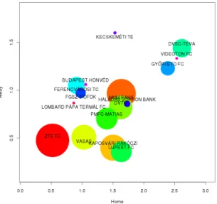
parametersλ1, λ2, λ3, ifX=Z1+Z3andY =Z2+Z3, whereZ1, Z2, Z3 follow independent Poisson distributions with parameters λ1, λ2, λ3, respectively. Clearly, X and Y are correlated with the correlation coefficient λ3. In our case, X and Y denote the number of goals scored by the home and away teams, respectively, whileZ3denotes the number of goals scored by both teams,Z1andZ2are the goal differences by which the match was won and lost, respectively, from the viewpoint of the home team. In the bivariate Poisson regression model, the intensity param- etersλ1, λ2, λ3depend on various covariates, e.g., the team indicators or the home playing indicator. The parameters incorporated by these covariates into the model are able to measure the impact of the home pitch or the team strength at home or away.

Algorithm 1 The EM algorithm for computing team scores.

Require: match_results:array of(home, away)team results anddesign_matrices:Xw, Xl, Xd;. The win, lose, and draw design matrices are defined by team-indicators and additional covariates.

Ensure: parameters:βw, βl, βd; .The parameters according to winning, losing, and drawing of the bivariate Poisson distribution.

1:procedureTeamScore(match_results,design_matrices,intensities) .Initialization

2: gd←min{home, away}; .Goals by both teams.

3: gw←home−gd; .Winning goals.

4: gl←away−gd; .Losing goals.

5: βw←glm(Xw, gw,"poisson"); .Fitting Poisson regression for winning goals by using theglm procedure.

6: βl←glm(Xl, gl,"poisson"); .Same for losing goals.

7: βd←glm(Xd, gd,"poisson"); .Same for draw.

8: λw←exp{Xw∗βw}; .Computing initial winning intensity.

9: λl←exp{Xl∗βl}; .Computing initial losing intensity.

10: λd←exp{Xd∗βd}; .Computing initial draw intensity.

11: repeat

.Expectation step 12: ^%←λd/(λw∗λl);

13: if(home >0)&(away >0)then

14: ^ratio←G[home, away]/G[home+ 1, away+ 1]; . Gis computed byCondExp 15: ^gd←home∗away∗%∗ratio;

16: else

17: ^gd←0;

18: end if

19: Repeat steps 3 and 4 with newgd; .Maximization step

20: Repeat steps 5, 6, and 7 with newgw, gl, gd; 21: Repeat steps 8, 9, and 10 with newβw, βl, βd; 22: untilconvergence;

23: returnλw, λl, λd; 24: end procedure

The parameters of bivariate Poisson regression are estimated by an EM-type algorithm, see Algorithm 1. This algorithm consists of two steps: the expectation (E) and the maximization (M) steps. In the E-step, the independent components Z1, Z2, Z3 are estimated from marginals X and Y using conditional expectation, see Algorithm 2. In the M-step, three separate Poisson regressions are fitted using the generalized linear model (GLM) framework. For example, this fitting can be done by using thefamily = poissonoption in theglmfunction of R. The output of Algorithm 1 can be, for example, the home, away, and draw strength of the teams in a league which can be shown as in Fig. 4 in the case of the Hungarian