Annales Mathematicae et Informaticae (51.)

(1)

ANNALES

MATHEMATICAE ET INFORMATICAE

TOMUS 51. (2020)

COMMISSIO REDACTORIUM

Sándor Bácsó (Debrecen), Sonja Gorjanc (Zagreb), Tibor Gyimóthy (Szeged), Miklós Hoffmann (Eger), József Holovács (Eger), Tibor Juhász (Eger), László Kovács (Miskolc), Gergely Kovásznai (Eger), László Kozma (Budapest), Kálmán Liptai (Eger), Florian Luca (Mexico), Giuseppe Mastroianni (Potenza),

Ferenc Mátyás (Eger), Ákos Pintér (Debrecen), Miklós Rontó (Miskolc), László Szalay (Sopron), János Sztrik (Debrecen), Gary Walsh (Ottawa)

HUNGARIA, EGER

(2)

MATHEMATICAE ET INFORMATICAE

VOLUME 51. (2020)

EDITORIAL BOARD

Sándor Bácsó (Debrecen), Sonja Gorjanc (Zagreb), Tibor Gyimóthy (Szeged), Miklós Hoffmann (Eger), József Holovács (Eger), Tibor Juhász (Eger), László Kovács (Miskolc), Gergely Kovásznai (Eger), László Kozma (Budapest), Kálmán Liptai (Eger), Florian Luca (Mexico), Giuseppe Mastroianni (Potenza),

Ferenc Mátyás (Eger), Ákos Pintér (Debrecen), Miklós Rontó (Miskolc), László Szalay (Sopron), János Sztrik (Debrecen), Gary Walsh (Ottawa)

INSTITUTE OF MATHEMATICS AND INFORMATICS ESZTERHÁZY KÁROLY UNIVERSITY

HUNGARY, EGER

(3)

(4)

11 ^th International Conference

on Applied Informatics

(5)

A kiadásért felelős az Eszterházy Károly Egyetem rektora Megjelent a Líceum Kiadó gondozásában

Kiadóvezető: Dr. Nagy Andor Felelős szerkesztő: Dr. Domonkosi Ágnes

Műszaki szerkesztő: Dr. Tómács Tibor Megjelent: 2020. július

(6)

(7)

(8)

Simulation results on a triangle-based network evolution model ^∗

István Fazekas, Attila Barta, Csaba Noszály

University of Debrecen fazekas.istvan@inf.unideb.hu

barta.attila@inf.unideb.hu noszaly.csaba@inf.unideb.hu

Submitted: February 4, 2020 Accepted: July 1, 2020 Published online: July 23, 2020

Abstract

We study a continuous time network evolution model. We consider the collaboration of three individuals. In our model, it is described by three connected vertices, that is by a triangle. During the evolution new collaborations, that is new triangles are created. The reproduction of the triangles is governed by a continuous time branching process. The long time behaviour of the number of triangles, edges and vertices is described. In this paper, we highlight the asymptotic behaviour of the network by simulation results.

Keywords:random graph, network, branching process, Malthusian parameter MSC:05C80, 90B15, 60J85

1. Introduction

In the past two decades network science became a popular and important topic, see [2]. It describes large real-life networks as the Internet, the WWW, social, biological and energy networks. Large networks have several common properties, therefore it is worth to study theoretical models of networks. Usually, networks are described by graphs. The nodes of the network are the vertices of the graph

∗This work was supported by the construction EFOP-3.6.3-VEKOP-16-2017-00002. The project was supported by the European Union, co-financed by the European Social Fund.

doi: 10.33039/ami.2020.07.005 https://ami.uni-eszterhazy.hu

7

(9)

and the connections are the edges. The meaning of connection can be cooperation or any interaction. A most cited paper in network science is [3]. It studies the famous preferential attachment model which leads to scale free networks. A deep mathematical study of discrete time network evolution models can be found in [6].

However, in our paper, we turn to a continuous time network evolution model.

An interesting continuous time model is presented in [7]. In that paper the theory of general branching processes, so called Crump-Mode-Jagers processes (see [8]) is applied to obtain asymptotic theorems. In paper [9], the idea of preferential attachment is combined with the evolution mechanism of a multi-type continuous time branching process.

In this paper we apply certain ideas of papers [1] and [7]. Paper [1] describes the interaction (or co-operation) of three persons. It creates a discrete time network evolution model which relies on the preferential attachment rule and three- interactions. In [7], however, a continuous time network evolution model based on a branching process evolution rule is presented. In that model only the usual interaction of two vertices is included and triangles have no role in the evolution rule. Neither [1] nor [7] offer numerical results. In our paper we combine the above ideas of three interactions with the continuous time branching process evolution mechanism. We focus on numerical studies of our model.

In this paper, in Section 2, we offer a detailed description of the evolution rules of our network. Then, in Section 3, we give a brief summary of our theoretical results. Their detailed mathematical proofs are given in a separate paper (see [5]).

Here, in Section 4, we present our numerical results. We show that our formulae are numerically tractable, so we can calculate the values of the important parameters and other features of our process. Then we show our simulation program and a certain part of our simulation results. These results support our mathematical theorems.

2. The network evolution model

We shall study the following evolving random graph model. At the initial time 𝑡= 0we start with a single triangle. During the evolution new triangles are born.

Every triangle has its own evolution process. We assume that during the evolution of the network the life processes of the triangles are identically distributed and independent of each other.

We denote the reproduction process of the generic triangle by𝜉(𝑡)and its birth times by 𝜏1, 𝜏2, . . .. We assume that 𝜏1, 𝜏2, . . . are the jumping time points of a Poisson processΠ(𝑡), 𝑡≥0, where the rate ofΠis equal to 1. Then the point process 𝜉(𝑡)gives the total number of offspring up to time𝑡. However, at a birth time not only triangles can be created but new edges and vertices can be added to the graph.

Here we describe the details of an evolution step. At every birth time 𝜏𝑖 a new vertex is added to the graph which can be connected to its ancestor triangle with𝑗 edges, where𝑗= 0,1,2,3. The vertices of the ancestor triangle to be connected to the new vertex are chosen uniformly at random. Let𝑝𝑗 denote the probability that

(10)

the new vertex will be connected to 𝑗 vertices of the ancestor triangle. It follows from the definition of the evolution process that at each birth step the possible number of the new triangles can be 0,1 or 3. On Figure 1 we represent these possibilities. The initial triangle is drawn by solid lines while the new ingredients by dashed lines. Denote the litter sizes belonging to the birth times 𝜏1, 𝜏2, . . . by

Figure 1: Possible birth events (0, 1, 2 or 3 new edges)

𝜀1, 𝜀2, . . .. Then𝜀1, 𝜀2, . . . are independent identically distributed discrete random variables with distribution P(𝜀𝑖=𝑗) =𝑞𝑗, 𝑗≥0. In our model the distribution of the litter size𝜀𝑖 is given by

P(𝜀𝑖= 0) =𝑞0=𝑝0+𝑝1, P(𝜀𝑖= 1) =𝑞1=𝑝2, P(𝜀𝑖= 3) =𝑞3=𝑝3, P(𝜀𝑖=𝑗) =𝑞𝑗= 0, if 𝑗 /∈ {0,1,3}.

We assume that the litter sizes are independent of the birth times 𝜏1, 𝜏2, . . ., too.

Denote by𝜆the life length of the generic triangle. 𝜆is a finite nonnegative random variable. After its death the triangle does not produce offspring, therefore 𝜉(𝑡) = 𝜉(𝜆)when𝑡 > 𝜆. Then the reproduction process of a triangle is

𝜉(𝑡) = ∑︁

𝜏𝑖≤𝑡∧𝜆

𝜀𝑖 =𝑆Π(𝑡∧𝜆),

where 𝑆𝑛 =𝜀1+· · ·+𝜀𝑛 gives the total number of offspring before the (𝑛+ 1)th birth event and𝑥∧𝑦 denotes the minimum of{𝑥, 𝑦}.

Let𝐿(𝑡)be the distribution function of𝜆. We assume that the survival function of the triangle’s life length is

1−𝐿(𝑡) =P(𝜆 > 𝑡) = exp

⎛

⎝−

∫︁𝑡 0

𝑙(𝑢) d𝑢

⎞

⎠,

where 𝑙(𝑡) is the hazard rate of the life span 𝜆. Moreover, we assume that the hazard rate depends on the number of offspring as

𝑙(𝑡) =𝑏+𝑐𝜉(𝑡) with positive constants𝑏and𝑐.

The whole evolution process is the following. The life and the reproduction process of the initial triangle is the same as that of the above described generic triangle.

When a child triangle is born, then it starts its own life and reproduction process which is also defined by the same way as its parent triangle. The same applies to

(11)

the grandchildren, etc. Therefore the evolution of the network is described by a continuous time branching process. We underline that the life and reproduction process of any triangle have the same distribution as those of the generic triangle, but the reproduction processes of different triangles are independent.

3. Theoretical results

Here we summarize the theoretical results of our paper [5].

Let 𝜇(𝑡) = E𝜉(𝑡) be the expectation of the number of offspring of a triangle up to time 𝑡. The total number of offspring of a triangle is 𝜉(∞). The expected offspring number of a triangle can be calculated as

𝜇(∞) =E𝜉(∞) = (𝑞1+ 3𝑞3)E(𝜆) = (𝑞1+ 3𝑞3)1

𝑐

∫︁1 0

(1−𝑢)^𝑏+1^𝑐⁻^𝑞⁰⁻¹𝑒^3𝑐^𝑢^(𝑞³^𝑢²^−3𝑞³^𝑢+3(𝑞¹^+𝑞³⁾⁾d𝑢.

The probability of extinction is1if𝜇(∞)≤1.

Theorem 3.1. If𝜇(∞)>1, then the probability of the extinction of the triangles is the smallest non-negative solution of equation

𝑞1+𝑞3(𝑦²+𝑦+ 1) 𝑐

∫︁1 0

(1−𝑢)^1+𝑏^𝑐⁻^𝑞⁰⁻¹𝑒⁽^𝑞¹^𝑦+𝑞³^𝑦

3

𝑐 𝑢−^𝑞³𝑐^𝑦³𝑢²+^𝑞³_3𝑐^𝑦³𝑢³)d𝑢= 1. (3.1) Assume that𝜇(∞)>1, that is our branching process is supercritical. Then the Malthusian parameter𝛼is the only positive solution of equation∫︀∞

0 𝑒⁻^𝛼𝑡𝜇(𝑑𝑡) = 1.

We can see that

𝑞1+ 3𝑞3−𝑏−1< 𝛼 < 𝑞1+ 3𝑞3−𝑏.

In our model the Malthusian parameter 𝛼satisfies the equation

1 = (𝑞1+ 3𝑞3) 𝑐

∫︁1 0

(1−𝑢)^{𝛼+(𝑏+1)}^𝑐 ⁻^𝑞^𝑐⁰⁻¹𝑒^3𝑞¹^𝑢+𝑞³^𝑢(𝑢

2−3𝑢+3)

3𝑐 d𝑢. (3.2)

Now we give the asymptotic behaviour of the number of triangles. Let us denote by 𝑍(𝑡)the number of triangles alive at time𝑡. Let𝛼be the Malthusian parameter.

Theorem 3.2. We have

𝑡→∞lim 𝑒^−𝛼𝑡𝑍(𝑡) =𝑌_∞𝑚_∞

almost surely and in𝐿¹, where the random variable𝑌_∞is nonnegative, it is positive on the event of non-extinction, it has expectation1 and

𝑚_∞= 1

(𝑞1+ 3𝑞3)²∫︀∞

0 𝑡𝑒⁻^𝛼𝑡(1−𝐿(𝑡))𝑑𝑡.

(12)

Now we turn to the asymptotic behaviour of vertices and edges. Let us denote by𝑉(𝑡)the total number of vertices (dead or alive) up to time𝑡. Let𝑊(𝑡)be the number of edges (dead or alive) up to time 𝑡. Let 𝛾 denote the number of new edges at a birth. Then its distribution isP(𝛾=𝑗) =𝑝𝑗, 𝑗= 0,1,2,3.

Theorem 3.3. We have 𝑉(𝑡) 𝑍(𝑡) → 1

𝛼 and 𝑊(𝑡)

𝑍(𝑡) → E𝛾 𝛼 as𝑡→ ∞almost surely on the event of non-extinction.

4. Numerical and simulation results

To get a closer look on the theoretical results, we made some simulations about them. We generated our code in Julia language [4]. We chose Julia, because of the great implementation of priority queues. The simulation time of our code was significantly faster in Julia than in other programming languages. We handled the main objects (the triangles) of our model as arrays with 3 elements. The elements were the indices of the edges that formed an individual for the process. We put all triangles in a priority queue with the priority of its birth time, because we can pop out the element with the lowest priority. After we have got the triangle with the lowest birth time, we can handle its birth process with the predefined parameters 𝑏, 𝑐, 𝑞1, 𝑞3. In the birth process we generated an exponential time step for the next birth step of our triangle. After that we checked if the triangle is still alive by calculating the survival function. If the triangle is dead, we move to the next one.

If it is alive, then we generate 1 or 3 new triangles and put them into the priority queue with the calculated birth time priorities. After this step we moved to the next birth event. The pseudocode of the birth process is seen at Algorithm 1.

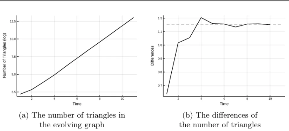
We made several simulation experiments. Here we show only some typical results. For the above demonstration first we used the parameter set 𝑏= 0.2, 𝑐= 0.2, 𝑝0 = 0.05, 𝑝1 = 0.05, 𝑝2 =𝑞1 = 0.6, 𝑝3 =𝑞3 = 0.3. On Figure 2a the solid curve shows the number of triangles. According to Theorem 3.2 it has asymptotic rate 𝑒^𝛼𝑡. Therefore we put logarithmic scale on the vertical axis, so the function 𝑍(𝑡)is a straight line for large values of𝑡. On the figure one can see that the shape of the curve is close to a straight line, so it supports our Theorem 3.2.

Then we checked the value of the Malthusian parameter𝛼. We can find it in two ways. On the one hand, the slope of the line on Figure 2a is𝛼for large values of the time. This slope can be approximated by the differences of the function. So on Figure 2b we present these differences (solid line). On the other hand, 𝛼can be calculated numerically from equation (3.2). This𝛼value is shown of Figure 2b by the horizontal dashed line. The fit of the differences to this 𝛼can be seen for large values of 𝑡. To get a closer look on the Malthusian parameter 𝛼, we fixed 5 parameter sets. Then we calculated 𝛼 from equation (3.2) for each case. It is shown in the fifth column of Table 1. Then for each of the parameter sets we

(13)

2 4 6 8 10 2.5

5.0 7.5 10.0 12.5

Time

Number of Triangles (log)

(a) The number of triangles in the evolving graph

2 4 6 8 10

0.7 0.8 0.9 1.0 1.1 1.2

Time

Differences

(b) The differences of the number of triangles Figure 2: Simulation results for𝑏= 0.2, 𝑐= 0.2, 𝑞1= 0.6, 𝑞3= 0.3

simulated our process𝑍(𝑡)five times. Then we calculated the differences oflog𝑍(𝑡) which should be good approximations of 𝛼according to Theorem 3.2. In Table 1,

̂︁

𝛼1, 𝛼̂︁2, ̂︁𝛼3, 𝛼̂︁4, 𝛼̂︁5 show the values of these approximations for large𝑡. One can see that each 𝛼̂︀𝑖 is close to the corresponding𝛼. We calculated numerically the

𝑏 𝑐 𝑞1 𝑞3 𝛼 ̂︁𝛼1 ̂︁𝛼2 ̂︁𝛼3 ̂︁𝛼4 ̂︁𝛼5

0.2 0.4 0.7 0.1 0.5628 0.5651 0.5730 0.5701 0.5611 0.5594 0.2 0.4 0.8 0.1 0.6531 0.6537 0.6497 0.6570 0.6510 0.6589 0.4 0.4 0.8 0.1 0.4531 0.4503 0.4519 0.4584 0.4541 0.4524 0.4 0.4 0.7 0.2 0.6545 0.6533 0.6517 0.6548 0.6534 0.6574 0.4 0.4 0.6 0.3 0.8535 0.8519 0.8489 0.8559 0.8547 0.8566

Table 1: ^𝛼from equation (3.2) and𝛼̂︀𝑖from simulations

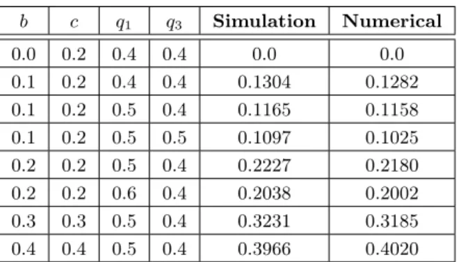
probability of extinction from equation (3.1). It is shown in the column ‘Numerical’

of Table 2. In the column ‘Simulation’ the relative frequency of the extinction is shown using our computer experiment. For each parameter sets, we simulated 10⁴ processes and counted the number of extinctions occured. The value of the relative frequency is close to the corresponding value of the probability in each case. So Table 2 supports the result of Theorem 3.1. To investigate how our difference process approximates 𝛼for large values of time𝑡, we simulated around 500 independent processes with the same parameters 𝑏 = 0.2, 𝑐 = 0.2, 𝑝0 = 0.05, 𝑝1 = 0.05, 𝑝2 = 𝑞1 = 0.6, 𝑝3 = 𝑞3 = 0.3 and same running time. Then we checked the differences of the last two values in the numbers of triangles that we simulated and made a histogram, seen in Figure 3. From equation (3.2) we obtained that the value of𝛼is0.3365. We see that the values of the differences are in [0.332,0.340], so they are very close to0.3365.

(14)

𝑏 𝑐 𝑞1 𝑞3 Simulation Numerical

0.0 0.2 0.4 0.4 0.0 0.0

0.1 0.2 0.4 0.4 0.1304 0.1282

0.1 0.2 0.5 0.4 0.1165 0.1158

0.1 0.2 0.5 0.5 0.1097 0.1025

0.2 0.2 0.5 0.4 0.2227 0.2180

0.2 0.2 0.6 0.4 0.2038 0.2002

0.3 0.3 0.5 0.4 0.3231 0.3185

0.4 0.4 0.5 0.4 0.3966 0.4020

Table 2: The relative frequency and the probability of the extinction of the triangles

Figure 3: Histogram of differences

To get some information about the random variable𝑌_∞𝑚_∞ represented in Theo- rem 3.2, we calculated the value of𝑍(𝑡)𝑒⁻^𝛼𝑡 for10³ independent repetitions of the process for the same time𝑡and same parameters 𝑞1= 0.3, 𝑞3= 0.6, 𝑏= 0.2, 𝑐= 0.2. On Figure 4 we represent the histogram and the empirical cumulative distribution function (ECDF) calculated from the simulation. We obtained that the empirical cumulative distribution function of𝑌_∞𝑚_∞ fits to a gamma distribution, as the Kolmogorov–Smirnov test gave us𝑝value 0.6713.

0 5 10 15 20

0.0 0.2 0.4 0.6 0.8

(a) Histogram of𝑍(𝑡)𝑒⁻^𝛼𝑡

0 5 10 15 20

0.00 0.25 0.50 0.75 1.00

(b) ECDF of𝑍(𝑡)𝑒⁻^𝛼𝑡 Figure 4: Simulation results for𝑍(𝑡)𝑒⁻^𝛼𝑡

(15)

5. Summary

In this paper and in [5] we offer a network evolution model which describes collaborations of 3 persons. Our model grasps certain features of real collaborations as emerging and disappearing collaborations, moreover collaborations of 2 persons are also allowed. Our numerical results confirm the theoretical ones. The present results prepare our future research on more complicated collaborations.

Algorithm 1 Birth process of a triangle

1: procedureBirth process

2: 𝑌 ←non-emptyPriority Queue

3: 𝑏, 𝑐, 𝑞1, 𝑞3←parameters of the survival function

4: 𝑥←dequeueY

5: if 𝑥is a new trianglethen

6: 𝑡0←the birth time of𝑥in the whole process

7: 𝑡←0, lifetime of𝑥

8: 𝑙←1, life variable

9: while𝑙= 1do

10: 𝑡←𝑡+𝐸𝑥𝑝(1)

11: 𝑝←the calculated survival function

12: if 𝑝 > 𝑈 𝑛𝑖(0,1)then

13: 𝑝0←𝑈 𝑛𝑖(0,1)

14: if 𝑝0< 𝑞1 then

15: take a new triangle with𝑡0+𝑡birth time to𝑌

16: offspring number is1at birth time𝑡

17: else if 𝑝0>1−𝑞3 then

18: take three new triangles with𝑡0+𝑡birth times to𝑌

19: offspring number is3at birth time𝑡

20: else

21: 𝑙←0

22: take 𝑡as the death time of𝑥to𝑌

References

[1] Á. Backhausz,T. F. Móri:A random graph model based on 3-interactions, Ann. Univ. Sci.

Budapest 36 (2012), pp. 41–52.

[2] A.-L. Barabási:Network science, Cambridge: Cambridge University Press, 2018.

[3] A.-L. Barabási,R. Albert:Emergence of scaling in random networks, Science 286.5439 (1999), pp. 509–512,

doi:https://doi.org/10.1126/fscience.286.5439.509.

[4] J. Bezanson,A. Edelman,S. Karpinski,V. B. Shah:Julia: A Fresh Approach to Nu- merical Computing, 2014, arXiv:1411.1607 [cs.MS].

(16)

[5] I. Fazekas,A. Barta,C. Nószály,B. Porvázsnyik:A continuous time evolution model describing 3-interactions, in: Manuscript, Debrecen, Hungary, 2020.

[6] R. van der Hofstad:Random Graphs and Complex Networks Vol. 1.Cambridge: Cambridge Series in Statistical and Probabilistic Mathematics, 2017,

doi:https://doi.org/10.1017/9781316779422.

[7] T. F. Móri,R. Sándor:A random graph model driven by timedependent branching dynam- ics, Ann. Univ. Sci. Budapest, Sect. Comp. 46.3 (2017), pp. 191–213.

[8] O. Nerman:On the convergence of supercritical general (C-M-J) branching processes, Z.

Wahrscheinlichkeitstheorie verw Gebiete 57 (1981), pp. 365–395, doi:https://doi.org/10.1007/BF00534830.

[9] S. Rosengren:A Multi-type Preferential Attachment Tree, Internet Math. 2018 (2018).

(17)

(18)

Numerical results on noisy blown-up matrices ^∗

István Fazekas, Sándor Pecsora

University of Debrecen, Faculty of Informatics fazekas.istvan@inf.unideb.hu pecsora.sandor@inf.unideb.hu

Submitted: February 4, 2020 Accepted: July 1, 2020 Published online: July 23, 2020

Abstract

We study the eigenvalues of large perturbed matrices. We consider an Hermitian pattern matrix𝑃 of rank𝑘. We blow up𝑃 to get a large block- matrix𝐵𝑛. Then we generate a random noise 𝑊𝑛 and add it to the blown up matrix to obtain the perturbed matrix 𝐴𝑛 = 𝐵𝑛+𝑊𝑛. Our aim is to find the eigenvalues of𝐵𝑛. We obtain that under certain conditions𝐴𝑛has 𝑘‘large’ eigenvalues which are called structural eigenvalues. These structural eigenvalues of𝐴𝑛 approximate the non-zero eigenvalues of𝐵𝑛. We study a graphical method to distinguish the structural and the non-structural eigenvalues. We obtain similar results for the singular values of non-symmetric matrices.

Keywords:Eigenvalue, symmetric matrix, blown-up matrix, random matrix, perturbation of a matrix, singular value

MSC:15A18, 15A52

1. Introduction

Spectral theory of random matrices has a long history (see e.g. [1, 5–8] and the references therein). This theory is applied when the spectrum of noisy matrices is

∗This work was supported by the construction EFOP-3.6.3-VEKOP-16-2017-00002. The project was supported by the European Union, co-financed by the European Social Fund.

17

(19)

considered. In [2] and [3] the eigenvalues and the singular values of large perturbed block matrices were studied. In [4] we extended the results of [2] and [3] and we suggested a graphical method to study the asymptotic behaviour of the eigenvalues. In this paper we consider the following important question for the numerical behaviour of the eigenvalues. How large the blown-up matrix should be in order to show the asymptotic behaviour given in the mathematical theorems? We also study the influence of the signal to noise ratio for our results.

Thus we consider a fixed deterministic pattern matrix𝑃, we blow up𝑃to obtain a ‘large’ block-matrix𝐵𝑛, then we add a random noise matrix𝑊𝑛. We present limit theorems for the eigenvalues of𝐴𝑛=𝐵𝑛+𝑊𝑛 as𝑛→ ∞and show corresponding numerical results. We also consider a graphical method to distinguish the structural and the non-structural eigenvalues. This test is important, because in real-life only the perturbed matrix 𝐴𝑛 is observed, but we are interested in eigenvalues or the singular values of 𝐵𝑛 which are approximated by the above mentioned structural eigenvalues/singular values of𝐴𝑛.

In Section 2 we list some theoretical results of [4]. In Section 3 the numerical results are presented. We obtained that the asymptotic behaviour of the eigenvalues can be seen for relatively low values of𝑛, that is if the block sizes are at least50, then we can use our asymptotic results. We also study the influence of the signal/noise ratio on the gap between the structural and non-structural singular values. Our numerical results support our graphical test visualised by Figure 1.

2. Eigenvalues of perturbed symmetric matrices

In this section we study the perturbations of Hermitian (resp. symmetric) blown-up matrices. We would like to examine the eigenvalues of perturbed matrices.

We use the following notation:

• 𝑃 is a fixed complex Hermitian (in the real valued case symmetric) 𝑘×𝑘 pattern matrix of rank𝑟

• 𝑝𝑖𝑗 is the(𝑖, 𝑗)’th entry of𝑃

• 𝑛1, . . . , 𝑛𝑘 are positive integers,𝑛=∑︀𝑘 𝑖=1𝑛𝑖

• 𝐵˜𝑛 is an𝑛×𝑛matrix consisting of𝑘²blocks, its block(𝑖, 𝑗)is of size𝑛𝑖×𝑛𝑗

and all elements in that block are equal to𝑝𝑖𝑗

• 𝐵𝑛 is called a blown-up matrix if it can be obtained from𝐵˜𝑛 by rearranging its rows and columns using the same permutation

Following [2], we shall use the growth rate condition

𝑛→ ∞ so that 𝑛𝑖/𝑛≥𝑐 for all 𝑖, (2.1) where 𝑐 > 0 is a fixed constant. Here we list those theorems of [4] which will be tested by numerical methods.

(20)

Proposition 2.1. Let 𝑃 be a symmetric pattern matrix, that is a fixed complex Hermitian (in the real valued case symmetric) 𝑘×𝑘 matrix of rank 𝑟. Let 𝐵𝑛 be the blown-up matrix of𝑃. Then𝐵𝑛 has𝑟non-zero eigenvalues. If condition (2.1) is satisfied, then the non-zero eigenvalues of𝐵𝑛 are of order𝑛 in absolute value.

Now, we assume that 𝑟𝑎𝑛𝑘(𝑃) = 𝑘. We shall consider the eigenvalues in descending order, so we have|𝜆1(𝐵𝑛)| ≥ · · · ≥ |𝜆𝑛(𝐵𝑛)|. Since 𝑘eigenvalues of 𝐵𝑛

are non-zero and the remaining ones are equal to zero, we shall call the first 𝑘 ones structural eigenvalues of 𝐵𝑛. Similarly, we shall call structural eigenvalue that eigenvalue of 𝐴𝑛, which corresponds to a structural eigenvalue of 𝐵𝑛. This correspondence will be described by Theorem 2.2 and Corollary 2.3. We shall see that the magnitude of any structural eigenvalue is large and it is small for the other eigenvalues.

First we consider perturbations by Wigner matrices. Next theorem is a gener- alization of Theorem 2.3 of [2] where the real valued case and uniformly bounded perturbations were considered.

Theorem 2.2. Let𝐵𝑛,𝑛= 1,2, . . ., be a sequence of complex Hermitian matrices.

Let the Wigner matrices 𝑊𝑛, 𝑛 = 1,2, . . ., be complex Hermitian 𝑛×𝑛 random matrices satisfying the following assumptions. Let the diagonal elements 𝑤𝑖𝑖 of 𝑊𝑛 be i.i.d. (independent and identically distributed) real, let the above diagonal elements be i.i.d. complex random variables and let all of these be independent. Let 𝑊𝑛 be Hermitian, that is𝑤𝑖𝑗 = ¯𝑤𝑗𝑖for all𝑖, 𝑗. Assume thatE𝑤₁₁² <∞,E𝑤12= 0, E|𝑤12−E𝑤12|²=𝜎² is finite and positive, E|𝑤12|⁴<∞. Then

lim sup

𝑛→∞

|𝜆𝑖(𝐵𝑛+𝑊𝑛)−𝜆𝑖(𝐵𝑛)|

√𝑛 ≤2𝜎

for all 𝑖almost surely.

Corollary 2.3. Let 𝐵𝑛, 𝑛= 1,2, . . ., be blown-up matrices of a complex Hermi- tian matrix 𝑃 having rank 𝑘. Assume that condition (2.1) is satisfied. Let the Wigner matrices 𝑊𝑛, 𝑛 = 1,2, . . ., satisfy the conditions of Theorem 2.2. Then Theorem 2.2 and Proposition 2.1 imply that𝐵𝑛+𝑊𝑛 has𝑘eigenvalues of order 𝑛 and the remaining eigenvalues are of order√𝑛almost surely.

So the structural eigenvalues have magnitude𝑛while the non-structural eigenvalues have magnitude√𝑛.

3. Singular values of perturbed matrices

In this section we study the perturbations of arbitrary blown-up matrices. We are interested in the singular values of matrices perturbed by certain random matrices.

We use the following notation:

• 𝑃 is a fixed complex 𝑎×𝑏pattern matrix of rank 𝑟

(21)

• 𝑝𝑖𝑗 is the(𝑖, 𝑗)’th entry of𝑃

• 𝑚1, . . . , 𝑚𝑎 are positive integers,𝑚=∑︀𝑎 𝑖=1𝑚𝑖

• 𝑛1, . . . , 𝑛𝑏 are positive integers,𝑛=∑︀𝑏 𝑖=1𝑛𝑖

• 𝐵˜𝑛 is an 𝑚×𝑛 matrix consisting of 𝑎×𝑏 blocks, its block (𝑖, 𝑗) is of size 𝑚𝑖×𝑛𝑗 and all elements in that block are equal to𝑝𝑖𝑗

• 𝐵𝑛 is called blown-up matrix if it can be obtained from𝐵˜ by rearranging its rows and columns

Following [3], we shall use the growth rate condition

𝑚, 𝑛→ ∞ so that 𝑚𝑖/𝑚≥𝑐 and𝑛𝑖/𝑛≥𝑑 for all 𝑖, (3.1) where 𝑐, 𝑑 > 0 are fixed constants. The following proposition is an extension of Proposition 6 of [3] to the complex valued case.

Proposition 3.1. Let 𝑃 be a fixed complex 𝑎×𝑏 matrix of rank 𝑟. Let 𝐵 be the 𝑚×𝑛 blown-up matrix of𝑃. If condition (3.1)is satisfied, then the non-zero singular values of 𝐵 are of order √𝑚𝑛.

Now we consider perturbation with matrices having independent and identically distributed (i.i.d.) complex entries. Let 𝑥𝑗𝑘, 𝑗, 𝑘 = 1,2, . . ., be an infinite array of i.i.d. complex valued random variables with mean 0and variance 𝜎². Let𝑋 = (𝑥𝑗𝑘)^𝑚,_{𝑗=1, 𝑘=1}^𝑛 be the left upper block of size𝑚×𝑛.

Theorem 3.2. For each𝑚and𝑛let𝐵 =𝐵𝑚𝑛 be a complex matrix of size𝑚×𝑛 and let 𝑋 =𝑋𝑚𝑛 be the above complex valued random matrix of size 𝑚×𝑛with i.i.d. entries. Moreover, assume that the entries of𝑋 have finite fourth moments.

Assume that 𝑚, 𝑛→ ∞so that 𝐾1≤ ^𝑚𝑛 ≤𝐾2, where0< 𝐾1≤𝐾2<∞are fixed constants. Denote by 𝑠𝑖 and 𝑧𝑖 the singular values of 𝐵 and𝐵+𝑋, respectively, 𝑠1≥ · · · ≥𝑠min{𝑚,𝑛},𝑧1≥ · · · ≥𝑧min{𝑚,𝑛}. Then for all 𝑖

|𝑠𝑖−𝑧𝑖|= O(√ 𝑛) as𝑚, 𝑛→ ∞ almost surely.

Corollary 3.3. Proposition 3.1 and Theorem 3.2 imply the following. Let 𝑃 be a fixed complex 𝑎×𝑏 matrix of rank 𝑟. Let 𝐵 be the 𝑚×𝑛 blown-up matrix of 𝑃. Assume that condition (3.1)is satisfied. Let𝑋 be complex valued perturbation matrices satisfying the assumptions of Theorem 3.2. Denote by 𝑧𝑖 the singular values of 𝐵+𝑋, 𝑧1 ≥ · · · ≥ 𝑧min{𝑚,𝑛}. Then 𝑧𝑖 are of order 𝑛 for 𝑖 = 1, . . . , 𝑟 and 𝑧𝑖 = O(√𝑛) for𝑖=𝑟+ 1, . . . ,min{𝑚, 𝑛} almost surely as 𝑚, 𝑛→ ∞ so that 𝐾1≤^𝑚𝑛 ≤𝐾2, where0< 𝐾1≤𝐾2<∞are fixed constants.

So the structural singular values (i.e. the largest 𝑟values) are ‘large’, and the remaining ones are ‘small’.

(22)

4. Numerical results

4.1. Eigenvalues of a symmetric matrix perturbed with Wigner noise

In [4] we concluded the following facts. In the case when the perturbation matrix has zero mean random entries, then the structural eigenvalues are ‘large’ and the non-structural ones are ‘small’. More precisely let|𝜆1| ≥ |𝜆2| ≥. . . be the absolute values of the eigenvalues of the perturbed blown-up matrix in descending order.

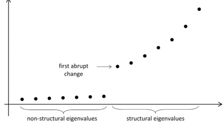
Then the structural eigenvalues|𝜆1| ≥ |𝜆2| ≥ · · · ≥ |𝜆𝑙|are ‘large’ and they rapidly decrease. The other eigenvalues|𝜆𝑙+1| ≥ |𝜆𝑙+2| ≥. . . are relatively small and they decrease very slowly. To obtain the structural eigenvalues we can use the following numerical (graphical) procedure. Calculate some eigenvalues of 𝐴𝑛 starting with the largest ones in absolute value. Stop when the last 5-10 eigenvalues are close to zero and they are almost the same in absolute value. Then we obtain the increasing sequence|𝜆𝑡| ≤ |𝜆𝑡−1| ≤ · · · ≤ |𝜆1|. Plot their values in the above order, then find the first abrupt change. If, say,

0≈ |𝜆𝑡| ≈ |𝜆𝑡−1| ≈ · · · ≈ |𝜆𝑙+1| ≪ |𝜆𝑙|<· · ·<|𝜆1|,

that is the first abrupt change is at 𝑙, then𝜆𝑙, 𝜆_𝑙−1, . . . , 𝜆1 can be considered as the structural eigenvalues. The typical abrupt change after the non-structural eigenvalues can be seen in Figure 1.

non-structural eigenvalues structural eigenvalues first abrupt

change

Figure 1: The abrupt change after the non-structural eigenvalues

Our first example supports Theorem 2.2 and Corollary 2.3 in the real valued case. The following results were obtained using the Julia programming language version 1.1.1. The simulations were divided into four steps. Let 𝑃 be the real

(23)

symmetric pattern matrix

⎡

⎢⎢

⎢⎣

8 7 2 5 3 2 4 0 3 1 7 9 6 3 4 0 2 5 2 0 2 6 7 6 5 4 2 0 3 4 5 3 6 8 7 6 0 5 4 2 3 4 5 7 9 8 8 6 5 1 2 0 4 6 8 7 6 8 0 4 4 2 2 0 8 6 9 7 6 6 0 5 0 5 6 8 7 8 8 4 3 2 3 4 5 0 6 8 9 6 1 0 4 2 1 4 6 4 6 5

⎤

⎥⎥

⎥⎦ .

In the initial step we have matrix𝑃. It has the following eigenvalues: 45.302, 15.497,10.914,7.677,−7.245,6.188,4.696,−3.789,−3.381and3.141. This matrix is blown up with the help of a vector containing the size informations of the blocks.

If the vector is n= [𝑛1, 𝑛2, . . . , 𝑛10], then the first row of blocks is built with the following block sizes: 𝑛1×𝑛1, 𝑛1×𝑛2, . . .𝑛1×𝑛10, the second row of blocks:

𝑛2×𝑛1, 𝑛2×𝑛2, . . .𝑛2×𝑛10 and we continue this pattern till the last row. In different simulations we used different vectorsnto blow up the matrix, it will be detailed separately for each simulation.

The next step is to generate the noise matrix, which is a symmetric real Wigner matrix, as defined in Section 2. The entries are generated in the following way: let the diagonal elements 𝑤𝑖𝑖 of 𝑊𝑛 be i.i.d. real with standard normal distribution, let the above diagonal elements be i.i.d. real random variables and let all of these be independent. The size of the noise matrix is equal to the size of the blown up matrix. After that, in order to obtain the noisy matrix, in each iteration we generate a new Wigner matrix and add to the blown up matrix.

As the last step we calculate the eigenvalues of the perturbed matrix. To do so we used theeigvalsfunction from theLinearAlgebrapackage. Julia provides native implementations of many common and useful linear algebra operations which can be loaded withusing LinearAlgebra, to install the package we usedusing Pkg and then with thePkg.add("LinearAlgebra")command we installed the package.

We studied 4 different schemes to blow up matrix𝑃, in each of these 4 schemes we applied 6 different block size vectors. These block series are given in Table 1.

We realised 1000 simulations for all block series in Table 1 and checked if the abrupt change like in Figure 1 was seen. For very low values of𝑛𝑖we did not find the abrupt change. In each case the first well distinguishable abrupt change appeared when𝑛1 was 50. This result is shown in Figures 2, 3, 4, and 5. At each figure the left side: |𝜆20(𝐴𝑛)| <· · · <|𝜆1(𝐴𝑛)|; right side: |𝜆20(𝐴𝑛)|<· · · <|𝜆6(𝐴𝑛)| in a typical realization in our example. The right side figures show only a part of the sequence around the change, so the jumps are clearly seen.

Each of the figures shows that there is an abrupt change between the11^th and 10^theigenvalues. So we can decide that the 10 largest eigenvalues are the structural

(24)

ones (which is the true value, since we used matrix𝑃 having rank 10).

Name of the scheme Series of the blocks

Equal

𝑛1=𝑛2=· · ·=𝑛10= 10 𝑛1=𝑛2=· · ·=𝑛10= 20 𝑛1=𝑛2=· · ·=𝑛10= 50 𝑛1=𝑛2=· · ·=𝑛10= 100 𝑛1=𝑛2=· · ·=𝑛10= 500 𝑛1=𝑛2=· · ·=𝑛10= 1000

Two types

𝑛1=𝑛2=· · ·=𝑛5= 10, 𝑛6=· · ·=𝑛10= 20 𝑛1=𝑛2=· · ·=𝑛5= 20, 𝑛6=· · ·=𝑛10= 40 𝑛1=𝑛2=· · ·=𝑛5= 50, 𝑛6=· · ·=𝑛10= 100 𝑛1=𝑛2=· · ·=𝑛5= 100, 𝑛6=· · ·=𝑛10= 200 𝑛1=𝑛2=· · ·=𝑛5= 500, 𝑛6=· · ·=𝑛10= 1000 𝑛1=𝑛2=· · ·=𝑛5= 1000, 𝑛6=· · ·=𝑛10= 2000

Arithmetic progression

𝑛1= 10, 𝑛2= 20, . . . , 𝑛10= 100 𝑛1= 20, 𝑛2= 30, . . . , 𝑛10= 110 𝑛1= 50, 𝑛2= 60, . . . , 𝑛10= 140 𝑛1= 100, 𝑛2= 110, . . . , 𝑛10= 190 𝑛1= 500, 𝑛2= 510, . . . , 𝑛10= 590 𝑛1= 1000, 𝑛2= 1010, . . . , 𝑛10= 1090

Four types

𝑛1=𝑛2= 10, 𝑛3=𝑛4=𝑛5= 20, 𝑛6=𝑛7=𝑛8= 30, 𝑛9=𝑛10= 40 𝑛1=𝑛2= 20, 𝑛3=𝑛4=𝑛5= 40, 𝑛6=𝑛7=𝑛8= 60, 𝑛9=𝑛10= 80 𝑛1=𝑛2= 50, 𝑛3=𝑛4=𝑛5= 100, 𝑛6=𝑛7=𝑛8= 150, 𝑛9=𝑛10= 200 𝑛1=𝑛2= 100, 𝑛3=𝑛4=𝑛5= 200, 𝑛6=𝑛7=𝑛8= 300, 𝑛9=𝑛10= 400 𝑛1=𝑛2= 500, 𝑛3=𝑛4=𝑛5= 1000, 𝑛6=𝑛7=𝑛8= 1500, 𝑛9=𝑛10= 2000 𝑛1=𝑛2= 1000, 𝑛3=𝑛4=𝑛5= 2000, 𝑛6=𝑛7=𝑛8= 3000, 𝑛9=𝑛10= 4000 Table 1: Schemes used to blow up matrix𝑃

(25)

0 2 4 6 8 10 12 14 16 18 20 0 500 1000 1500 2000 2500

6 7 8 9 10 11 12 13 14 15 16 17 18 19 20 0 50 100 150 200 250 300 350

Figure 2: Equal: 𝑛1=𝑛2=· · ·=𝑛10= 50

0 2 4 6 8 10 12 14 16 18 20 0 500 1000 1500 2000 2500 3000 3500 4000

6 7 8 9 10 11 12 13 14 15 16 17 18 19 20 0 50 100 150 200 250 300 350 400 450 500 550

Figure 3: Two types: 𝑛1=· · ·=𝑛5= 50,𝑛6=· · ·=𝑛10= 100

0 2 4 6 8 10 12 14 16 18 20 0 500 1000 1500 2000 2500 3000 3500 4000 4500 5000

6 7 8 9 10 11 12 13 14 15 16 17 18 19 20 0 100 200 300 400 500 600 700

Figure 4: Arithmetic progression: 𝑛1= 50, 𝑛2= 60, . . . , 𝑛10= 140

0 2 4 6 8 10 12 14 16 18 20 0 1000 2000 3000 4000 5000 6000 7000

6 7 8 9 10 11 12 13 14 15 16 17 18 19 20 0 100 200 300 400 500 600 700 800

Figure 5: Four types: 𝑛1=𝑛2= 50, 𝑛3=𝑛4=𝑛5= 100, 𝑛6=𝑛7=𝑛8= 150, 𝑛9=𝑛10= 200

(26)

As the block’s sizes are increasing, the border between the structural and non- structural eigenvalues is getting more and more significant, as it is shown in Fig- ure 6. We see, that when𝑛𝑖 = 1000(for all𝑖), then the gap is much larger than in the case of 𝑛𝑖= 50.

0 2 4 6 8 10 12 14 16 18 20 0 0.5 1 1.5 2 2.5 3 3.5 4 4.5

5 10⁴

6 7 8 9 10 11 12 13 14 15 16 17 18 19 20 0 1000 2000 3000 4000 5000 6000 7000

Figure 6: Equal: 𝑛1=𝑛2=· · ·=𝑛10= 1000

In Table 2, we list the averages of the absolute values of the eigenvalues making 1000 repetitions in each case. More precisely,𝑛𝑖means that all blocks were𝑛𝑖×𝑛𝑖

and in the column below𝑛𝑖 there are the 20 largest of the averages of the absolute values of the corresponding eigenvalues of different 𝐴𝑛 matrices. We see, that there is a gap between the10^th and 11^th values even in the relatively small value of 𝑛𝑖 = 10. The larger the value of 𝑛𝑖, the larger the gap. This table shows that our test is very reliable for moderate (e.g. 𝑛𝑖= 50) sizes of the blocks.

𝑗 𝑛𝑖= 10 𝑛𝑖= 20 𝑛𝑖= 50 𝑛𝑖= 100 𝑛𝑖= 200 𝑛𝑖= 500 𝑛𝑖= 1000 1 453.26 906.28 2265.40 4530.50 9060.70 22652.00 45303.00 2 155.64 310.65 775.43 1550.31 3100.00 7748.90 15497.00 3 110.06 219.28 546.65 1092.40 2183.90 5458.00 10915.00

4 77.99 154.82 385.08 768.93 1536.70 3839.60 7677.90

5 73.76 146.21 363.63 725.90 1450.40 3624.10 7246.90

6 63.36 125.32 310.93 620.41 1239.20 3095.40 6189.40

7 48.86 95.95 236.92 471.66 941.21 2349.90 4697.80

8 40.51 78.39 192.04 381.54 760.54 1897.10 3791.70

9 36.30 70.32 171.90 340.95 678.98 1693.20 3383.40

10 34.06 65.84 160.18 317.23 631.47 1573.90 3144.70

11 18.56 27.21 44.03 62.73 89.04 141.14 199.78

12 17.96 26.70 43.58 62.33 88.67 140.84 199.50

13 17.45 26.27 43.20 61.99 88.37 140.58 199.27

14 17.03 25.92 42.90 61.72 88.14 140.38 199.09

15 16.65 25.59 42.62 61.47 87.92 140.18 198.92

16 16.33 25.28 42.36 61.25 87.72 140.01 198.77

17 15.99 25.00 42.11 61.03 87.53 139.85 198.63

18 15.69 24.74 41.89 60.83 87.34 139.69 198.49

19 15.40 24.47 41.67 60.64 87.17 139.54 198.36

20 15.12 24.23 41.47 60.45 87.01 139.40 198.23

Table 2: Eigenvalues in the case of equal size blocks

(27)

4.2. Singular values of a non-symmetric perturbed matrix

This example supports Theorem 3.2 and Corollary 3.3. Let 𝑃 be the 7×8 real non-symmetric pattern matrix

⎡

⎢⎢

⎣

6 5 6 5 3 2 1 2 3 9 6 7 4 5 6 1 4 8 9 8 3 4 2 1 5 7 6 8 7 5 3 2 2 5 7 8 9 6 5 3 1 3 4 5 6 7 6 4 2 1 4 6 7 8 9 9

⎤

⎥⎥

⎦ .

In the previous example we showed the effect of the blocks’ sizes, now we show the effect of the signal to noise ratio (snr) on the singular values of 𝑃. To blow up 𝑃, we chose block heights as [𝑚1, . . . , 𝑚𝑎] = [500,750,500,600,750,550,500]

and block widths as[𝑛1, . . . , 𝑛𝑏] = [500,500,600,1000,550,500,550,500]. Then we blew up𝑃, and we added a noise to get the perturbed matrix. Like in Section 3, we denote by 𝐵 the blown-up matrix which is the signal, by 𝑋 the noise matrix, and by𝐴=𝐵+𝑋 the perturbed matrix. We shall use the following definition of the signal to noise ratio

snr=

1 𝑚𝑛

∑︀𝑚 𝑖=1

∑︀𝑛 𝑗=1𝑏²_𝑖,𝑗

1 𝑚𝑛

∑︀𝑚 𝑖=1

∑︀𝑛 𝑗=1𝑥²_𝑖,𝑗. Here 𝑚=∑︀𝑎

𝑖=1𝑚𝑖 is the number of rows, 𝑛=∑︀𝑏

𝑗=1𝑛𝑗 is the number of columns in 𝐵 and𝑋,𝑏𝑖,𝑗 is the element of the signal matrix𝐵, while𝑥𝑖,𝑗 is the element of the noise matrix𝑋 in the𝑖^th row and𝑗^th column.

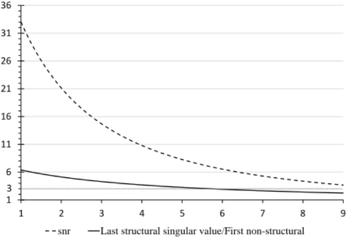
In this example, the entries of the noise matrix𝑋 are independent and, at the initial step, they are from standard normal distribution. In each of the following steps we increased the noise, by multiplying each of the elements of the noise matrix by certain multipliers. The first multiplier was 1.002, the second one was1.004, then1.006, . . . ,3.000.

So, during the experiment, we amplify the noise step-by-step and check at each iteration the snr and the ratio of the last (smallest) structural singular value and the first (largest) non-structural one. If the structural/non-structural ratio reaches a certain point, the signal gets so noisy, that it is not possible any more to distinguish the structural singular values from the non-structural ones. On Figure 7 the dashed line is the signal to noise ratio and the solid line is the ratio of the the last (smallest) structural singular value and the first (largest) non-structural singular value. On the horizontal axis the scale is given by the variance of the noise. One can see, that when the noise grows, then the snr decreases quickly, but the structural/non-structural ratio decreases quite slowly. If the structural/non- structural ratio decreases close to 1, then we reach a point, where the structural and non-structural singular values are not well distinguishable any more. However, Figure 7 shows that our method is reliable, that is if the noise in not higher than

(28)

25%of the signal, then the structural singular values are well distinguishable from the non-structural ones.

1 6 11 16 21 26 31 36

1 2 3 4 5 6 7 8 9

snr Last structural singular value/First non-structural 3

Figure 7: Signal to noise ratio compared to structural/non-structural singular value ratio

5. Conclusion

The shown graphical method works appropriately to distinguish the structural and non-structural eigenvalues and singular values. The size of the blocks has an influence on the ‘jump’ between the non-structural and the structural eigenvalues.

As the block’s sizes are increasing, the border between the structural and non- structural eigenvalues is getting more and more significant. If the block sizes are at least 50, then the structural and the non-structural eigenvalues are well distinguishable. Our test is reliable, if the noise is less than 25%, but above this noise level it can be unreliable.

References

[1] Z. D. Bai:Methodologies in spectral analysis of large dimensional random matrices. A review.

Statistica Sinica 9 (1999), pp. 611–677.

[2] M. Bolla:Recognizing linear structure in noisy matrices.Linear Algebra and its Applications 402 (2005), pp. 228–244,

doi:https://doi.org/10.1016/j.laa.2004.12.023.

[3] M. Bolla,A. Krámli,K. Friedl:Singular value decomposition of large random matrices (for two-way classification of microarrays).J. Multivariate Analysis 101.2 (2010), pp. 434–

446,

doi:https://doi.org/10.1016/j.jmva.2009.09.006.

[4] I. Fazekas,S. Pecsora:On the spectrum of noisy blown-up matrices.Special Matrices 8.1 (2020), pp. 104–122,

doi:https://doi.org/10.1515/spma-2020-0010.

(29)

[5] Z. Füredi,J. Komlós:The eigenvalues of random symmetric matrices.Combinatorica 1 (1981), pp. 233–241,

doi:https://doi.org/10.1007/BF02579329.

[6] S. O’Rourke,D. Renfrew:Low rank perturbations of large elliptic random matrices.Elec- tron. J. Probab 19 (2014), pp. 1–65,

doi:https://doi.org/10.1214/EJP.v19-3057.

[7] T. Tao:Outliers in the spectrum of iid matrices with bounded rank perturbations.Probability Theory and Related Fields 155 (2013), pp. 231–263,

doi:https://doi.org/10.1007/s00440-011-0397-9.

[8] H. V. Van:Spectral norm of random matrices.Combinatorica 27 (2007), pp. 721–736, doi:https://doi.org/10.1007/s00493-007-2190-z.

(30)

Indoor localization simulation framework for optimized sensor placement to increase

the position estimation accuracy

Ádám Kaló, Zoltán Kincses, László Schäffer, Szilveszter Pletl

University of Szeged, Department of Technical Informatics

Kalo.Adam@stud.u-szeged.hu,{kincsesz,schaffer,pletl}@inf.u-szeged.hu Submitted: February 4, 2020

Accepted: July 1, 2020 Published online: July 23, 2020

Abstract

Indoor position estimation is an important part of any indoor application which contains object tracking or environment mapping. Many indoor localization techniques (Angle of Arrival – AoA, Time of Flight – ToF, Return Time of Flight – RToF, Received Signal Strength Indicator – RSSI) and technologies (WiFi, Ultra Wideband – UWB, Bluetooth, Radio Frequency Identi- fication Device – RFID) exist which can be applied to the indoor localization problem. Based on the measured distances (with a chosen technique), the position of the object can be estimated using several mathematical methods.

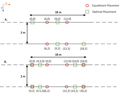
The precision of the estimated position crucially depends on the placement of the anchors, which makes the position estimate less reliable. In this paper a simulation framework is presented, which uses genetic algorithm and the multilateral method to determine an optimal anchor placement for a given pathway in an indoor environment. In order to make the simulation more re- alistic, the error characteristics of the DWM1001 UWB ranging module were measured and implemented in the simulation framework. Using the proposed framework, various measurements with an optimal and with a reference anchor placement were carried out. The results show that using an optimal anchor placement, a higher position estimation accuracy can be achieved.

Keywords:Anchor placement, Ultra Wide Band, Multilateral, Genetic Algo- rithm, Indoor Localization, Non-linear Measurement Error Model

29

(31)

1. Introduction

The location of a device or user can be effectively obtained outdoor using the Global Positioning System (GPS), but it could be challenging in an indoor environment. During the last decade, indoor localization has been investigated mainly for wireless sensor networks and robotics. However, nowadays, the wide-scale usage of mobile phones and wearable devices has enabled localization in a wide range of applications like health-care, industry, surveillance and home management.

In the literature many localization technologies and techniques are available [9].

A Received Signal Strength Indicator (RSSI), which is the strength of the signal received usually measured in decibel-milliwatts (dBm), and a wireless Ethernet based localization approach is used in [4]. Using a path-loss model and the RSS, the distance between the sender and receiver can be estimated. In [7] an Angle of Arrival (AoA) and Wireless LAN (Wifi) based method is applied using an antennae array for the estimation of the angle by computing the difference between the arrival times at the individual elements of the array. A Time of Flight (ToF) and 2.4 GHz radio based approach is presented in [5], using signal propagation time to compute the distance between the transmitter and the receiver. A similar technique, the Return Time of Flight (RToF) is used in conjunction with RSSI in a Wifi-based method in [10].

RToF is a two-way ranging method where the transmitter sends a ranging mes- sage to the receiver at 𝑡1 time. The receiver sends it back with a delay of 𝑡_proc time and it arrives to the original transmitter at 𝑡2 time. The time of flight is 𝑡2−𝑡1−𝑡_proc, and the distance can be calculated with the speed of the signal, depending on the technology. The accuracy of the measurement highly depends on 𝑡proc.

The UWB is a recently researched communication technology providing more accurate ToF and RToF estimations. It uses ultra-short pulses with a time period less than a nanosecond, resulting in a low duty cycle which leads to lower power consumption. Its frequency range is from 3.1 to 10.6 GHz with a bandwidth of 500 MHz. Since the UWB usually operates at a low energy level, typically between

−40 and −70dB, most of the other technologies detect it as background noise.

This makes it practically immune to interference with other systems since it has a radically different signal type and radio spectrum. Moreover, the signal (especially in its lower frequencies) can penetrate through walls because signal pulses are very short. Utilizing this attribute, it is easier to differentiate the main path from the multi-paths, providing more accurate estimations [8].

Once the point-to-point distances between the objects are measured, the un- known position of the object can be estimated. There are various algebraic methods to estimate the position from the point-to-point distances like triangulation or mul- tilateration. Most of them require a few devices with known fixed positions (anchor nodes) to calculate the actual position of the moving device (mobile node). In case of error-free distance measurements, these methods theoretically give an exact position. But real distance measurements contain errors which depend on the relative