Contents
T. Ásványi, Representation transformations of ordered lists . . . 5 Á. Baran, Gy. Terdik, Power spectrum estimation of spherical random
fields based on covariances . . . 15 M. Cserép, D. Krupp,Component visualization methods for large legacy
software in C/C++ . . . 23 J. H. Davenport,Solving computational problems in real algebra/geomet-
ry . . . 35 J. H. Davenport, What does Mathematical Notation actually mean, and
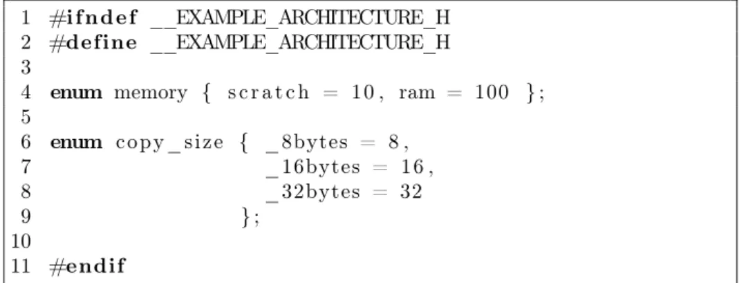
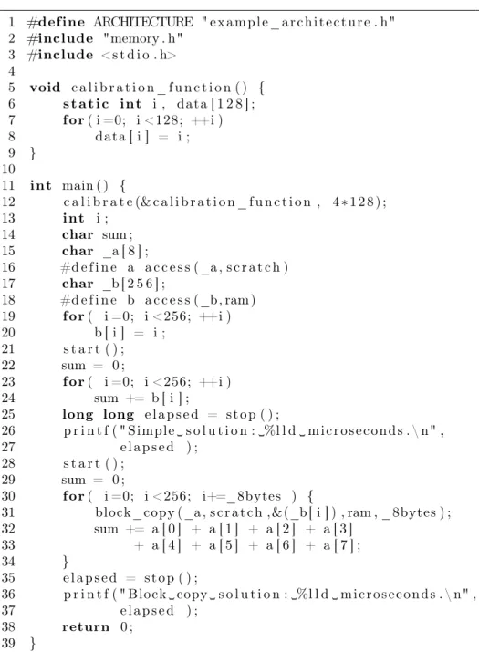
how can computers process it? . . . 47 G. Dévai,Lightweight simulation of programmable memory hierarchies . . . 59 I. Fazekas, S. Pecsora, A generalization of the Barabási-Albert random
tree . . . 71 Z. Gál, T. Tajti, Gy. Terdik,Surprise event detection of the supercom-
puter execution queues . . . 87 G. Horváth, N. Pataki, Clang matchers for verified usage of the C++
Standard Template Library . . . 99 P. Kasza, P. Ligeti, Á. Nagy,On a secure distributed data sharing system
and its implementation . . . 111 Gy. Kocsisné Szilágyi, A. Kocsis, A special localization algorithm in
Wireless sensor networks for telemetry application . . . 121 A. London, T. Németh, A. Pluhár, T. Csendes, A local PageRank
algorithm for evaluating the importance of scientific articles . . . 131 G. Rácz, Z. Pusztai, B. Kósa, A. Kiss,An improved Community-based
Greedy algorithm for solving the influence maximization problem in social networks . . . 141 T. Radványi, Cs. Biró, S. Király, P. Szigetváry, P. Takács, Survey
of attacking and defending in the RFID system . . . 151 Z. Ruzsa, Zs. Parisek, R. Király, T. Tómács, T. Szakács, H. Haja-
gos,Building of a mathematics-based RFID localization framework . . 165 J. R. Sendra, S. M. Winkler, Optimization of coefficients of lists of
polynomials by evolutionary algorithms . . . 177 J. Sütő, S. Oniga, A. Buchman, Real time human activity monitoring . . 187 P. Takács, Z. E. Csajbók, T. Mihálydeák,Boundaries of membrane in
P systems relying on multiset approximation spaces in language R . . . 197
ANNALESMATHEMATICAEETINFORMATICAE44.(2015)
ANNALES
MATHEMATICAE ET INFORMATICAE
TOMUS 44. (2015)
COMMISSIO REDACTORIUM
Sándor Bácsó (Debrecen), Sonja Gorjanc (Zagreb), Tibor Gyimóthy (Szeged), Miklós Hoffmann (Eger), József Holovács (Eger), László Kovács (Miskolc),
László Kozma (Budapest), Kálmán Liptai (Eger), Florian Luca (Mexico), Giuseppe Mastroianni (Potenza), Ferenc Mátyás (Eger),
Ákos Pintér (Debrecen), Miklós Rontó (Miskolc), László Szalay (Sopron), János Sztrik (Debrecen), Gary Walsh (Ottawa)
HUNGARIA, EGER
ANNALES MATHEMATICAE ET INFORMATICAE International journal for mathematics and computer science
Referred by
Zentralblatt für Mathematik and
Mathematical Reviews
The journal of the Institute of Mathematics and Informatics of Eszterházy Károly College is open for scientific publications in mathematics and computer science, where the field of number theory, group theory, constructive and computer aided geometry as well as theoretical and practical aspects of programming languages receive particular emphasis. Methodological papers are also welcome. Papers sub- mitted to the journal should be written in English. Only new and unpublished material can be accepted.
Authors are kindly asked to write the final form of their manuscript in LATEX. If you have any problems or questions, please write an e-mail to the managing editor Miklós Hoffmann: hofi@ektf.hu
The volumes are available athttp://ami.ektf.hu
MATHEMATICAE ET INFORMATICAE
VOLUME 44. (2015)
EDITORIAL BOARD
Sándor Bácsó (Debrecen), Sonja Gorjanc (Zagreb), Tibor Gyimóthy (Szeged), Miklós Hoffmann (Eger), József Holovács (Eger), László Kovács (Miskolc),
László Kozma (Budapest), Kálmán Liptai (Eger), Florian Luca (Mexico), Giuseppe Mastroianni (Potenza), Ferenc Mátyás (Eger),
Ákos Pintér (Debrecen), Miklós Rontó (Miskolc), László Szalay (Sopron), János Sztrik (Debrecen), Gary Walsh (Ottawa)
INSTITUTE OF MATHEMATICS AND INFORMATICS ESZTERHÁZY KÁROLY COLLEGE
HUNGARY, EGER
9 th International Conference
on Applied Informatics
HU ISSN 1787-6117 (Online)
A kiadásért felelős az Eszterházy Károly Főiskola rektora Megjelent az EKF Líceum Kiadó gondozásában
Kiadóvezető: Czeglédi László Műszaki szerkesztő: Tómács Tibor Megjelent: 2015. június Példányszám: 30
Készítette az
Eszterházy Károly Főiskola nyomdája Felelős vezető: Kérészy László
Representation transformations of ordered lists ∗
Tibor Ásványi
Eötvös Loránd University, Faculty of Informatics Budapest, Hungary
asvanyi@inf.elte.hu
Submitted September 15, 2014 — Accepted March 5, 2015
Abstract
Search and update operations of dictionaries have been well studied, due to their practical significance. There are many different representations of them, and some applications prefer this, the others that representation. A main point is the size of the dictionary: for a small one a sorted array can be the best representation, while for a bigger one an AVL tree or a red-black tree might be the optimal choice (depending on the necessary operations and their frequencies), and for an extra large one we may prefer a B+-tree, for example.
Consequently it can be desirable to transform such a collection of data from one representation into another, efficiently. There is a common feature of the data structures mentioned: they can be considered strictly ordered lists. Thus in this paper we start a new topic of interest: How to transform a strictly ordered list form one representation into another, efficiently? What about the time and space complexities of such transformations?
Keywords:strictly increasing list, representation-transformation, data struc- ture (DS), linear, array, binary tree (BT), balanced, search tree
MSC:68P05, 68P10, 68P20, 68Q25
1. Introduction
In this paper we consider strictly increasing lists. They can be represented in several different ways. For example, with alinear data structure (LDS)(e.g. array,
∗Supported by Eötvös Loránd University, Faculty of Informatics.
http://ami.ektf.hu
5
linked list, sequential file), with abinary search tree (BST)(e.g. unbalanced BST, AVL tree, red-black tree), with aB-tree,B+-tree, etc. [1, 2, 3].
Their common features are that they can be traversed increasingly in Θ(n) time: the linear traversal of a LDS has linear operational complexity; similarly, the inorder traversal of a tree needsΘ(n)time. And the search-and-update operations can run in O(n)time. [1, 2]
In this paper we use three asymptotic computational complexity measures (each time we consider the worst case by default): O(g(n))(upper bound),Ω(g(n))(lower bound), andΘ(g(n)) =O(g(n))∩Ω(g(n))[2].
Sorted arrayssupport only the search with O(log(n))operational complexity, but for the balanced search tree1 representations each of thesearch, insert, delete operations have this complexity. On linked lists, and sequential files we cannot perform any search-and-update operation inO(log(n))time. Thus we concentrate on the sorted array, and balanced search tree representations of such lists. The search, insert, delete operations have been well studied. Sometimes we have to transform these lists from one representation into another. Consequently we pay attention to these representation-transformations. We ask, how to transform a strictly ordered list Lfrom one representation into another,efficiently?
Undeniably, the operational complexity of such a transformation isΩ(n): each item must be processed. In some cases, it is also O(n): Undoubtedly, a linear representation ofLcan be produced inO(n)time, because the input representation ofLcan be traversed also inO(n)time. Thus, regardless of the input representation of L, a linear representation ofL can be generated withΘ(n)atomic operations.
Besides, a balanced search tree representation ofLcan be generated inO(nlog(n)) time, because a single insert needsO(log(n))atomic operations. Nevertheless this method does not use the information that the input issorted.
Consequently this is our question: Given an input representation ofL, when and how can we produce a balanced search tree representation of it, with an operational complexityΘ(n), or at least better thanΘ(nlog(n))? We give a partial answer to this question. We invent three algorithms. With operational complexityΘ(n), we transform (1) astrictly increasing arrayinto anAVLtree; (2) astrictly increasing array into ared-blacktree; (3) anAVLtree into ared-blacktree.
2. Main results
In order to expound these algorithms (a) we define size-balanced BSTs, and an algorithm transforming astrictly increasing array into such a size-balanced BST;
(b) we prove that a size-balanced BST is almost complete, and so (c) it is anAVL tree; (d) we colour the almost complete BSTs asred-blacktrees; (e) we find a special property ofAVLtrees, and invent an algorithm colouring them as red-blacktrees.
(a-c) are needed for transforming astrictly increasing array into an AVL tree (Section 2.1). (a,b,d) result in the transformation of astrictly increasing arrayinto
1AVL tree, red-black tree, SBB-tree, rank-balanced tree, B-tree, B+-tree, etc.
ared-blacktree (Section 2.2). The theorems and algorithm of (e) in Subsection 2.3 form the high point of this section.
2.1. Strictly increasing array to AVL tree
First we enumerate the necessary notions. By trees we mean rooted ordered trees [2]. Remember thatN IL is the empty tree. The leaves of a nonempty tree have no child. The non-leaves are the internal nodes.
Ift6=N ILis a binary tree (BT),left(t)is its left andright(t)is its right subtree.
If t is a BT, s(t) is its size, i.e. s(t) = 0, if t =N IL; s(t) = 1 +s(left(t)) + s(right(t)), otherwise. h(t) is its height, i.e. h(t) = −1, if t = N IL; h(t) = 1 + max(h(left(t)), h(right(t))), otherwise.
If r is the root node of a BT t 6= N IL, left(r) = left(t), right(r) = right(t), and root(t) =r. Provided thattis a BT,n∈t,ifft6=N IL∧(n= root(t)∨n∈ left(t)∨n∈right(t)).
dt(n)is the depth of nodenin BTt. Ift6=N IL,dt(root(t)) = 0. Ifnis a node of a BT t and left(n) 6= N IL, dt(root(left(n))) = dt(n) + 1. If right(n) 6= N IL, dt(root(right(n))) = dt(n) + 1. Node n is strictly binary (SB(n)), iff left(n) 6= N IL∧right(n)6=N IL.
Clearly, h(t) = max{dt(n) | n ∈ t}, if t 6= N IL. A BT t is complete, iff (∀n∈t)(dt(n)< h(t)→SB(n)).
Notice that for any leafnof a complete BTt,d(n) =h(t); ands(t) = 2h(t)+1−1. A BTtisalmost complete(AC(t)),iff(∀n∈t)(dt(n)< h(t)−1→SB(n)).
Notice that a BT isAC, iffcompared to the appropriate complete BT, nodes may be missing only from its lowest level: Figure 1 shows such a tree. Clearly, for a leaf nof anAC BTt,dt(n)∈ {h(t), h(t)−1}. The nodes oftat depthh(t)−1 may have one or two children, or may be leaves. s(t)∈[2h(t),2h(t)+1−1].
---7---
/ \
---4--- ---10----
/ \ / \
2 5 9 12
/ \ / \ / \ / \
1 3 NIL NIL 8 NIL 11 NIL
Figure 1: almost complete BST: the places of the missing nodes are shown by NILs
A noden of a BT is height-balanced,iff|h(right(n))−h(left(n))| ≤1. A BT t is height-balanced, iff(∀n ∈t), n is height-balanced. An AVL tree is a height- balanced BST.
A noden of a BT is size-balanced,iff|s(right(n))−s(left(n))| ≤1. A BT t is size-balanced,iff(∀n∈t), nis size-balanced.
We transform a strictly increasing array into an equivalent size-balanced BST in linear time:
We take the middle item of a nonempty array. This will label the root node of the tree. Next we transform the left and right sub-arrays into the appropriate subtrees, recursively. An empty array is transformed into an empty tree.
The resulting size-balanced BST is also an AVL tree, as it follows from the next two theorems.
Theorem 2.1. A size-balanced binary tree is also almost complete (AC).
Proof. We use mathematical induction with respect to the height h(t)of the size- balanced tree t. If h(t) = −1, then t is empty, and AC(t). Let us suppose that we have this property for trees with h(t) ≤ h. Let h(t) = h+ 1. Then t 6= N IL∧h(left(t)) ≤ h∧h(right(t)) ≤ h. It follows by induction that left(t) and right(t)are almost complete. Also|size(left(t))−size(right(t))| ≤1. (Furthermore, remember that a complete binary tree of height hhas the size 2h+1−1, and an almost complete binary tree with size in[2h+1,2h+2−1]has heighth+ 1.) Now we enumerate the possible cases about the subtrees oft, and prove thatAC(t)in each case. If the two (almost complete) subtrees have the same size, their heights are also equal, andAC(t). If the smaller subtree is complete, then the bigger one has an extra leaf at its extra level, and AC(t). If the smaller subtree is not complete, then the bigger one has the same height, andAC(t).
Theorem 2.2. An almost complete binary tree is also height-balanced.
Proof. We can suppose t 6= N IL. First, if AC(t), the leaves of t have depth h(t)or h(t)−1. Thus h(left(t)), h(right(t))∈ {h(t)−1, h(t)−2}. Consequently,
|h(right(t))−h(left(t))| ≤1. As a result,root(t)is balanced. Next, let us suppose thatlr(t)∈ {left(t),right(t)}. Now, ifAC(t), then(∀n∈lr(t))(dt(n)< h(t)−1→ SB(n)). Therefore (∀n ∈ lr(t))(dlr(t)(n) < h(t)−2 → SB(n)). We also have h(lr(t))≤h(t)−1. For these reasons(∀n∈lr(t))(dlr(t)(n)< h(lr(t))−1→SB(n)).
As a result, AC(lr(t)). Thus each (direct or indirect) subtree of t is AC, and if a subtree is nonempty, its root node is balanced. Finally, each node of t is balanced.
Corollary 2.3. A size-balanced BST is also an AVL tree.
Proof. A size-balanced BST is almost complete, thus height-balanced.
Consequently, the algorithm we defined above transforms a strictly increasing array into an equivalent AVL tree. It takes Θ(n)time, because each item of the array is processed once. Besides the Θ(n) size of its output, it needs Θ(log(n)) working memory: this is the height of the recursion. Provided that we need the heights of the nonempty subtrees in their root nodes (as it is usual with AVL trees), we can return the height of a subtree when we return from the appropriate recursive call, and compute the height of a subtree with a given root node from the heights of the two subtrees of that node.
2.2. Strictly increasing array to red-black tree
We have an algorithm transforming a strictly increasing array into an almost com- plete BST. We also have the height of the tree. Here we need an additional flag showing whether the tree is complete or not. Clearly, a nonempty BT is complete, iff its too subtrees are also complete, and their heights are the same. Thus the computation of this flag is also easily merged into the algorithm above.
Next, if we prove that an almost complete BST (with its height and flag) can be coloured in linear time, as a red-black tree, then we have also the algorithm transforming a strictly increasing array into such a tree.
Definition 2.4. A red-black tree is a BST with red and black nodes: The root node is black. We regard NILs as pointers to black, external leaves. For each node, all simple paths from the node to descendant NIL-leaves contain the same number of black nodes. If a node is red, then both its children are black. [2] (See Figure 2.)
---BLACK---
/ \
----red---- --BLACK--
/ \ / \
BLACK BLACK red NIL
/ \ / \ / \
NIL NIL NIL NIL NIL NIL
Figure 2: Red-black tree
Based on this definition, the algorithm of colouring is simple: consider the complete levels of an almost complete BST, and paint the nodes black. If the tree is not complete, the nodes at the lowest, partially filled level remain, and we paint them red. (See Figure 3.) Unquestionably this procedure needs Θ(n) time and Θ(log(n))working memory. The algorithm computing its input (the almost complete tree, its height, and flag) has the same measures. Consequently, the whole transformation has these time and space requirements.
---BLACK---
/ \
---BLACK--- --BLACK--
/ \ / \
red red red NIL
/ \ / \ / \
NIL NIL NIL NIL NIL NIL
Figure 3: Almost complete tree painted as red-black tree
2.3. AVL tree to red-black tree
We colour an AVL tree t as a red-black tree. We use a postorder and a preorder traversal. As a result, our procedure needsΘ(n)time andΘ(log(n))(proportional to the height of t) working memory [1].
Definition 2.5. Minimal height of a binary tree t: m(t) = −1, if t = N IL;
1 + min(m(left(t)), m(right(t))), otherwise.
Theorem 2.6. If t is a height-balanced tree thenm(t)≤h(t)≤2m(t) + 1. Proof. It comes with mathematical induction with respect tom(t). Ifm(t) =−1⇒ t=N IL⇒h(t) =−1⇒m(t)≤h(t)≤2m(t) + 1. Let us suppose that we have this property for trees with m(t) = k. Let m(t) = k+ 1. We can suppose that m(left(t)) =k. By induction: k≤h(left(t))≤2k+1. The treetis height-balanced.
Therefore h(right(t)) ≤ 2k+ 2. Thus k+ 1 ≤ 1 + max(h(left(t)), h(right(t))) = h(t)≤2k+ 3 = 2(k+ 1) + 1. As a result: m(t)≤h(t)≤2m(t) + 1. (Notice that m(t)≤h(t)for any binary tree.)
In thecolouringalgorithm, first we calculatem(t). Based on the definition, this can be done with a postorder traversal oft. In a typical AVL tree, for each non-NIL subtree soft, theh(s)attributes are already present. (If not, the computation of theh(s)values can be easily merged into the postorder traversal.)
Next, with a preorder traversal of t, we colour t. (See Figure 4). We paint m(t) + 1nodes black on each simple path from the root to a NIL-leaf. (The NIL- leaves are also considered black, but we do not paint them.)
PreCondition of the first call:
I0: t is AVL tree and b = m(t)+1 and
h(s) is calculated for each subtree s of t procedure colour( t : BinTree; b : integer )
/* I1: b>=0 and b-1 =< m(t) and h(t) =< 2*b */
if( t \= NIL ) {
/* Note: paint b nodes black on each branch of t */
if( h(t) < 2*b ) { colour(t) := black b := b-1 }
else /* I2: 0 =< b =< m(t) and h(t) = 2*b */
colour(t) := red colour(left(t),b) colour(right(t),b) } end of procedure colour
Figure 4: Colouring an AVL treetas a red-black tree
Now we are going to prove the correctness of thecolouringalgorithm in Figure 4.
Terminology: In the rest of this section we useI0(i.e. the PreCondition), invari- antsI1,I2, and other logical statements. Let us suppose thatIj, Ik∈ {I0, I1, I2}; P,Qare arbitrary statements. When we say thatIj withP inducesIkwithQ, we mean: IfIj andP are true when the program is at the place ofIj, thenIkandQ will hold when the run of the program next time arrives at the place ofIk.
Lemma 2.7. I0 inducesI1 withh(t)<2b.
Proof. Based on the definition of m(t), m(t) ≥ −1. Consequently b = m(t) + 1 impliesb≥0∧b−1≤m(t). Theorem 2.6 impliesh(t)≤2m(t) + 1. Considering b=m(t)+1we receiveh(t)≤2m(t)+1 = 2(b−1)+1 = 2b−1. Thush(t)<2b. Lemma 2.8. I1 with t6=N IL∧h(t)<2b inducesI1 in both recursive calls.
Proof. Lets(t)be the left or right subtree parameterizing the appropriate recursive call. Thus we need to prove I1b←b−1,t←s(t) i.e. that the following three conditions hold:
(1) b−1 ≥0: We know thath(t)≥0 (since t 6=N IL) and h(t) <2b. Conse- quently,b >0, and thereforeb−1≥0.
(2) b−2 ≤ m(s(t)): From I1, b−1 ≤ m(t). From the definition of m(t), m(t)≤1 +m(s(t)). As a result, b−1≤1 +m(s(t)), i.e. b−2≤m(s(t)). (3) h(s(t)) ≤ 2(b−1): h(t) < 2b, i.e. h(t) ≤ 2b−1; h(s(t)) ≤ h(t)−1; thus
h(s(t))≤2b−2.
Lemma 2.9. I1 with t6=N IL∧h(t)≥2b inducesI2.
Proof. h(t)≤2b andh(t)≥2bimpliesh(t) = 2b. 0≤b remains true. Considering Theorem 2.6 we have2b≤2m(t) + 1; thusb≤m(t) + 1/2 i.e.b≤m(t).
Lemma 2.10. I2 inducesI1with h(t)<2b in both recursive calls.
Proof. Lets(t)be the left or right subtree parameterizing the appropriate recursive call. Thus we have to prove (I1∧h(t)<2b)t←s(t) i.e. b ≥0∧b−1 ≤m(s(t))∧ h(s(t))<2b. b≥0 remains true. Fromb≤m(t)andm(t)≤1 +m(s(t))we have b−1≤m(s(t)). h(t) = 2bimpliesh(s(t))<2b.
Theorem 2.11. Provided that the precondition I0 holds, procedure colour paints the nodes of tree t so thatt becomes a red-black tree.
Proof. Lemmas 2.7, 2.8, 2.9, and 2.10 imply that I1 andI2 are invariants of the program. I1means that when we arrive at an external leaf, i.e.t=N IL,0≤b≤ m(t) + 1 =−1 + 1, as a resultb= 0. In the programbis decreased (by 1), exactly when a node is painted black. Because b is decreased to zero on each branch of any subtree while we go to a NIL-leaf, we have the same number of black nodes on these paths. Lemma 2.7 implies that the root node of the tree is painted black.
Lemma 2.10 makes sure that both children of a red node will also be black. These have the effect of receiving a red-black tree.
Let acrb-tree be a BST which can be coloured as a red-black tree. Then an AVL tree is also a crb-tree. This also follows from both of the following results.
(1) Bayer proved that the class ofSBB-treesproperly contains the AVL trees [4], and we know from 4.7.2 in [3] that the SBB-trees and the red-black trees are structurally equivalent.
(2) Rank-balanced trees are a relaxation of AVL trees, and form a proper subclass of crb-trees [5].
Our achievements and these results are unrelated. In this subsection our contribu- tions are the notion of the minimal height of an AVL tree, theorems 2.6 and 2.11, and ourefficient colouring algorithmproved.
3. Conclusions
This was our question: How to transform a strictly increasing list L from one representation into another,efficiently?
Summarizing this paper, we already know that given an input representation of L, we can produce another representation of it in Θ(n)time, if this other rep- resentation is a linear data structure, an AVLor red-blacktree. In some cases we have direct transformations, in other cases we need a temporary array.
In three cases we invented the necessary algorithms, theorems, lemmas, and proofs. The first two, (sorted array →balanced BST) programs create new trees;
but the second half of the second algorithm, and the third (AVL tree→red-black tree) procedure do not make structural changes on the actual tree, just paint its nodesblack, andred. Each of the three programs needsΘ(log(n))working memory.
Our algorithms and theorems imply three relations among four classes of BSTs:
size-balanced BSTs ⊂ almost complete BSTs ⊂ AVL trees ⊂ crb-trees. Actually, each of the first three classes is a proper subclass of the next one. For exam- ple2 BST (((1)2(3))4(5)) is almost complete, but not size-balanced; AVL tree ((((1)2)3(4))5(6(7)))is not almost complete; red-black tree((1b)2b((3b)4r(5b(6r)))) is not height-balanced.
Open questions: IfLis transformed into another type of balanced search trees (notinto an AVL orred-black tree); for example, into a B-tree, we know that the operational complexity of the transformation is Ω(n), and O(nlog(n)). Here we still need more sharp results. Maybe, from a strictly increasing list, each kind of balanced search trees can be generated inΘ(n)time? Are there some cases, when the time complexity is more thanΘ(n), but less thanΘ(nlog(n))?
If the input representation ofLis a search tree (or a linked list or a sequential file), and the output is anAVLor red-blacktree, we can make the transformation in Θ(n) time, but – with the exception of theAVL tree→red-black tree program
2Using the notation(left-subtree root right-subtree)where the empty subtrees are omitted.
– we actually need a temporary array, thusΘ(n)working space. We ask: In which cases can we reduce the memory needed?
References
[1] Weiss, Mark Allen, Data Structures and Algorithm Analysis, Addison-Wesley, 1995, 1997, 2007, 2012, 2013.
[2] Cormen, T.H., Leiserson, C.E., Rivest, R.L., Stein, C.,Introduction to Algo- rithms,The MIT Press, 2009. (Ebook: http://bit.ly/IntToAlgPDFFree)
[3] Wirth, N., Algorithms and Data Structures,Prentice-Hall Inc., 1976, 1985, 2004.
(Ebook: http://www.ethoberon.ethz.ch/WirthPubl/AD.pdf)
[4] Bayer R.,Symmetric Binary B-Trees: Data Structure and Maintenance Algorithms, Acta Informatica 1, 290–306 (1972),Springer-Verlag, 1972.
[5] Haeupler B., Sen S., Tarjan R.E., Rank-Balanced Trees, Algorithms and Data Structures: 11th International Symposium, WADS 2009, Banff, Canada, August 2009, pp 351–362,Springer-Verlag, LNCS 5664, 2009.
Power spectrum estimation of spherical random fields based on covariances ∗
Ágnes Baran, György Terdik
Faculty of Informatics, University of Debrecen baran.agnes@inf.unideb.hu
terdik.gyorgy@inf.unideb.hu
Submitted September 15, 2014 — Accepted November 20, 2014
Abstract
A Gaussian isotropic stochastic field on a 2D-sphere is characterized by either its covariance function or its angular spectrum. The object of this paper is the estimation of the spectrum in two steps. First we estimate the covariance function, secondly we approximate the series expansion of the covariance function with respect of Legendre polynomials. Simulations show that this method is fast and precise.
Keywords:Angular correlation, angular spectrum, isotropic fields on sphere, estimation of correlation
MSC:60G60, 62M30
1. Introduction
There are several physical phenomena which can be described with the help of a spherical random processes. A typical example of random data measured on the surface of a sphere is the cosmic microwave background radiation (CMB). Similar random fields arise in medical imaging, in analysis of gravitational and geomagnetic data etc.. These fields are characterized by a series expansion with respect to the spherical harmonics. Under assumption of Gaussianity both the covariance function and the angular power spectrum describe completely the probability structure of
∗The publication was supported by the TÁMOP-4.2.2.C-11/1/KONV-2012-0001 project. The project has been supported by the European Union, co-financed by the European Social Fund.
http://ami.ektf.hu
15
an isotropic stochastic field. The estimated spectrum can be used to check the underlying physical theory, while the possible non-Gaussianity can be investigated by estimating the higher order angular spectra.
1.1. Notations
LetS2denote the surface of the unit sphere inR3, andX(L)be a random field on S2, where the locationL= (ϑ, ϕ), andϑ∈[0, π]is the co-latitude, whileϕ∈[0,2π]
is the longitude. If the spatial processX(L)is mean square continuous, then it has a series expansion in terms of spherical harmonics Y`m. Spherical harmonics are defied by the Legendre polynomials
P`(x) = 1 2``!
d`
dx`(x2−1)`, x∈[−1,1], (`= 0,1,2, . . .) and the associated Legendre functions
P`m= (−1)m(1−x2)m/2 dm dxmP`(x),
of degree ` and order m, where ` = 0,1,2, . . ., and m = −`, . . . , `. Now the complex valued spherical harmonics of degree ` and orderm (` = 0,1,2, . . ., and m=−`, . . . , `) are given by
Y`m(ϑ, ϕ) =λm` (cosϑ)eimϕ, where
λm` (x) =
s2`+ 1 4π
(`−m)!
(`+m)!P`m(x), ifm≥0, and
λm` (x) = (−1)mλ|m|` (x), ifm <0, that implies
Y`−m(ϑ, ϕ) = (−1)mY`m(ϑ, ϕ).
Using these notations the spherical harmonics expansion of the random field X(L)∈L2(S2)is
X(L) = X∞
`=0
X` m=−`
Z`mY`m(L), where the coefficients
Z`m, `= 0,1, . . . , m=−`, . . . , `
are complex valued centered random variables, while puttingEZ00=µimplies that EX(L) =µand the coefficients are given by
Z`m= Z
S2
X(L)Y`m(L)dL, (1.1)
and
Z`m= (−1)mZ`−m.
2. Spectrum
Definition. The random fieldX(L)is called strongly isotropic if all finite dimen- sional distributions of{X(L), L∈S2} are invariant under the rotationg for every g∈SO(3), whereSO(3)denotes the special orthogonal group of rotations defined onS2.
If the spatial processX is strongly isotropic, then E(Z`m11Z`m22) =f`1δ`1`2δm1m2
for `1, `2 ∈N, and mi =−`i, . . . , `i, whereδ`k = 1 if ` = k and zero otherwise, while
E(Z00Z`m) = f0+E(Z00)2
δ0`δ0m, f0=V ar Z00 .
f` =V ar(Z`m), `= 0,1,2, . . ., are nonnegative real numbers, and (f`, `∈ N0) is called the angular power spectrum of the random fieldX. Note E(X) =µ, hence C2(L1, L2) =E(X(L1)−µ)(X(L2)−µ)is the covariance function of the isotropic field X(L). Due to the isotropy the covarianceC2(L1, L2)depends on the angular distanceγ of the locationsL1 andL2 only (wherecosγ=L1·L2). That means
C2(L1, L2) =C2(gL2L1L1, N) =:C(cosγ),
where gL2L1 is the rotation which takesL2into the north pole N andL1into the planexOz.
It is straightforward (see [5]) that
C(cosγ) = X∞
0
f`
2`+ 1
4π P`(cosγ). (2.1)
For the practical computation of the spectrumfkthe orthogonality of the Legendre polynomials can be used: witht= cos(γ)from (2.1) follows
Z1
−1
C(t)P`(t)dt=f`2`+ 1 4π
Z1
−1
[P`(t)]2dt=f`· 1 2π, that is
f`= 2π Z1
−1
C(t)P`(t)dt, (2.2)
for`= 0,1,2, . . ..
Example (Lapalce-Beltrami model on S2). Consider the homogeneous isotropic field X onR3according to the equation
4 −c2
X =∂W, where 4 = ∂x∂22
1 +∂x∂22 2 +∂x∂22
3, denotes the Laplace operator on R3. Its spectrum, see ([6]), is
S(λ) = 2 (2π)2
λ2
(λ2+c2)2, λ2=k(λ1, λ2, λ3)k2, with covariance of Matérn Class
C(r) = 1 (2π)3/2
(cr)1/2K1/2(cr)
2c ,
whereK1/2 is the modified Bessel (Hankel) function, see [1].
Now according to the Lapalce-Beltrami operator, which is the restriction of4onto the unit sphereS2,
4B = 1 sinϑ
∂
∂ϑ
sinϑ ∂
∂ϑ
+ 1
sin2ϑ
∂2
∂ϕ2, we consider the stochastic model
4B−c2
XB =∂WB,
on sphere. The covariance function C0 of XB is the restriction of the covariance functionC ofX on sphere andC0(cosγ) =C(2 sin (γ/2)), i.e.
C0(cosγ) = 1 (2π)3/2
rsin (γ/2)
2c K1/2(2csin (γ/2)).
We apply the Poisson formula whenΦ (dλ) =S(λ)dλ, and we obtain the spectrum forXB
f`= 2π2 Z∞ 0
J`+1/22 (λ)1 λ
2 (2π)2
λ2 (λ2+c2)2dλ
= Z∞ 0
J`+1/22 (λ) λ
(λ2+c2)2dλ.
3. HEALPix
The most widely used pixelisation of the sphere for sampling and analyzing CMB data is the HEALPix (Hierarchical, Equal Area and isoLatitude Pixelization), see
[2]. Actually the CMB data are given on the surface of a unit ball at the discrete points defined by HEALPix. Here in the base resolution partitioning the surface of the sphere is divided into12quadrilateral pixels of same area, and in each further resolution the pixels are subdivided into 4 equal area pixels. Denoting by Nside
the resolution parameter, the total number of pixels equals12Nside2 , and the pixel centers are located on4Nside−1isolatitude rings. Unfortunately, the pixelisation is not rotational invariant, the pixel centers can be rotated into each other in the case of some rotations around the north-south axes only.
4. Computational results
Let us suppose that we are given an observation of an isotropic field on the sphere, more precisely for each HEALPix pixelLwe have a valueX(L). The estimator of the spectrum of the field can be based either on (1.1) or on (2.1). It means that we can approximate the integral (1.1), then for each fixed` we estimatef` as the variance of approximatedZ`m,m=−`, . . . , `. In this case one can not expect good result for small `, since the estimator of the variance f` based on 2`+ 1 values.
The alternative method is based on the estimation of covariance function first then use the expansion (2.1) according to the Legendre polynomials for estimatingf`. The advantage of this later one is that there are many distances between pixels in which the estimation of the covariance is possible.
For further improvement of this computations we are going to apply some sam- pling theorems concerning on spherical harmonics and Legendre polynomials. We show this method through simulations.
In our simulations we consider random fields not only with zero mean but with f0 = 0 as well. The reason is that we have only one realization and when we center the observation the sample mean contains a value ofZ00hencef0can not be identified.
To the numerical approximation of the integral (2.2) denote byt1, t2, . . . , tn the nodes of the quadrature (−1≤ti≤1), and for a givenilet(Li1j, Li2j),j= 1, . . . , N, be pairs of pixels which have angular distanceti. Considering the samples
X1, X2, . . . , XN, where Xj =X(Li1j), and
Y1, Y2, . . . , YN, where Yj=X(Li2j), we use the empirical covariance
Cbi= 1 N
XN j=1
XjYj
to estimate the valueC(ti),i= 1, . . . , n.
In the program we used only pixels located in the equatorial area (i.e. pixel centers with co-latitude −13 ≤ cosϑ ≤ 13). E.g. in the case of Nside = 16these
pixels determine nearly 9000 different values for t. In the equatorial zone each ring contains the same number of pixels (4Nside), moreover the pixel centers are equidistant located. In order to calculate the possible values of t = cosγ we considered the first pixel center on each ring in the north equatorial belt together with the pixel centers located on and below the actual ring. More precisely it is suffices to consider on each ring only the half of the pixels. After that for a given t to collect the pixel-pairs having distance t we can use the rotation symmetry.
Depending on the location of the original pixel-pair (L1, L2), which was used to compute t, there exist4Nside, 8Nside or 16Nside pairs having the given distance.
If both of the pixels lie on the equator, or θ1 = π−θ2 and ϕ1 = ϕ2 (where L1 = (θ1, ϕ1),L2= (θ2, ϕ2)), that is the locations are symmetric to the equator, then the number of pairs is equal to4Nside. In the case ofθ1=θ26=π2 and in the case of θ16=π−θ2 and ϕ1 =ϕ2, moreover ifθ1 =π−θ2 andϕ1 6=ϕ2, there are 8Nsidepairs. In all other cases there exist16Nsidepairs corresponding to the given distance.
By the numerical calculation of (2.2) using the Gaussian quadrature instead of the built-in Matlab functiontrapz enables a more efficient calculation, since these method requires much less evaluations of empirical covariances, however, this could be subject of further investigations.
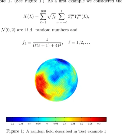
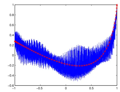
Test example 1. (See Figure 1.) As a first example we considered the spatial process
X(L) = X100
`=1
pf`
X` m=−`
Z`mY`m(L), (4.1)
whereZ`m∼ N(0,2) are i.i.d. random numbers and
f`= 1
(`(`+ 1) + 4)2, `= 1,2, . . .
−0.2 −0.15 −0.1 −0.05 0 0.05 0.1 0.15 0.2 0.25 0.3
Figure 1: A random field described in Test example 1
By the discretization of the sphere we usedNside= 16as resolution parameter, which results 3072 pixels located on 63 isolatitude rings.
The estimated and theoretical correlations can be seen on Figure 2 such that f0=f1= 0.
−1 −0.5 0 0.5 1
−0.6
−0.4
−0.2 0 0.2 0.4 0.6 0.8 1
Figure 2: Estimated correlation in Test example 1
Let us denote byfˆ`,`= 1, . . . ,100the estimated spectrum, then we obtained X100
`=1
(f`−fˆ`)2≈1.93·10−4 and
1≤max`≤100|f`−fˆ`|= 4.2·10−3.
Test example 2. In the second example we investigated the field defined by the sum (4.1) taking
f`= 4π
2`+ 10.8`, `= 1,2, . . .
The covariance is estimated from the generated field, and the theoretical correlation
C(γ) = 1
p1−1.6 cosγ+ 0.82 −1;
are shown on Figure 3.
−1 −0.5 0 0.5 1
−0.8
−0.6
−0.4
−0.2 0 0.2 0.4 0.6 0.8 1
Figure 3: Estimated correlation in Test example 2
References
[1] Abramowitz, M., Stegun, I.A.,Handbook of mathematical functions with formu- las, graphs and mathematical tables,Dover Publications Inc., New York, (1992) [2] Górski, K.M., Hivon, E., Banday, A. J., Wandelt, B.D., Hansen, F.K.,
Reinecke, M., Bartelmann, M., HEALPix: A framework for high-resolution dis- cretization and fast analysis of data distributed on the sphere, The Astrophysical Journal, Vol. 622 (2005), 759–771.
[3] Lang, A., Schwab, C.,Isotropic Gaussian Random Fields on the Sphere, Regularity, Fast Simulation, and Stochastic Partial differential Equations,arXiv:1305.1170v1 [4] Marinucci, D., Peccati, G.,Random fields on the Sphere, Cambridge University
Press, Cambridge, (2011)
[5] Terdik, Gy.,Angular Spectra for non-Gaussian Isotropic Fields,arXiv:1302.4049v2, to appear Brazilian Journal of Probability and Statistics,http://imstat.org/bjps/
papers/BJPS249.pdf
[6] Yadrenko, M. I.,Spectral theory of random fields,Optimization Software Inc. Pub- lications Division, New York, (1983)
Component visualization methods for large legacy software in C/C++
Máté Cserép
a, Dániel Krupp
baEötvös Loránd University mcserep@caesar.elte.hu
bEricsson Hungary daniel.krupp@ericsson.com
Submitted August 28, 2014 — Accepted February 24, 2015
Abstract
Software development in C and C++ is widely used in the various in- dustries including Information Technology, Telecommunication and Trans- portation since the 80-ies. Over this four decade, companies have built up a huge software legacy. In many cases these programs, implementing complex features (such as OS kernels, databases) become inherently complicated and consist of millions lines of code. During the many years long development, not only the size of the software increases, but a large number (i.e. hundreds) of programmers get involved. Mainly due to these two factors the maintenance of software becomes more and more time consuming and costly.
To attack the above mentioned complexity issue, companies apply various source code cross-referencers to help in the navigation and visualization of the legacy code. In this article we present a visualization methodology that helps programmers to understand the functional dependencies of artifacts in the C++ code in the form similar to UML component diagrams. Our novel graph representation reveals relations between binaries, C/C++ implementation files and headers. Our technique is non-intrusive. It does not require any modification of the source code or any additional documentation markup. It solely relies on the compiler generated Abstract Syntax Tree and the build information to analyze the legacy software.
Keywords:code comprehension, software maintenance, static analysis, com- ponent visualization, graph representation, functional dependency
MSC:68N99 http://ami.ektf.hu
23
1. Introduction
One of the main task of code comprehension software tools is to provide naviga- tion and visualization views for the reusable elements of the source code, because humans are better at deducing information from graphical images [2, 7]. We can identify reusable software elements in C/C++ language on different abstraction levels of modularity. At a finer granularity, functions provide reusable implemen- tation of a specific behavior, while on a higher scale (in C++) classes defines the next level, where a programmer can collect related functions and data that belong to the same subject-matter. At the file level, header files group related functions, variables, type declarations and classes (in C++ only) into a semantic unit.
State of the art software comprehension and documentation tools implement various visualization methods for all of these modularization layers. For example, on the function level call graph diagrams can show the relations between the caller and the called functions [9], while on the class level, one can visualize the contain- ment, inheritance and usage relations by e.g. UML diagrams. On the file level, header inclusion diagrams help the developers in code comprehension [8].
However, our observations showed that the state of the art file level diagrams are not expressive enough to reveal some important dependency relationships among implementation and header files. In this paper, we describe a new visualization methodology that exposes the relations between implemented and used header files and the source file dependency chains of C/C++ software.
This paper is structured as follows. Section 2 consist of a brief overview of the state of the art literature with special focus on static software analysis. In Section 3 we describe the shortfalls of the visualization methods in the current software comprehension tools, then in Section 4 we present our novel views that can help C and C++ programmers in understanding legacy source code. Section 5 demonstrates our results by showing examples on real open-source projects, and finally in Section 6 we conclude the paper and set the directions for future work.
2. Background
Researchers have proposed several software visualization techniques and various taxonomies have been published over the past years. They address one or more of three main aspects (static, dynamic, and evolutional) of a software. The visu- alization of the static attributes focuses on displaying the software at a snapshot state, dealing only with the information that is valid for all possible executions of the software, assisting the comprehension of the architecture of the program.
Conversely, the visualization of the dynamic aspects shows information about a particular execution of the software, therefore helps to understand the behavior of the program. Finally, the visualization of the evolution – of the static aspects – of a software handles the notion of time, visualizing the alternations of these attributes through the lifetime of the software development. For a comprehensive summary of the current state of the art see the work of Caserta et al.[3]
The static analysis of a software can be executed on different levels of granularity based on the level of abstraction. Above a basic source code level, a middle – package, class or method – level, and an even higher architecture level exists.
In each category a concrete visualization technique can focus on various different aspects. A summary of categorization is shown on Table 1, classifying some of the most known and applied, as well as a few interesting new visualization techniques.
Kind Level Focus Techniques
Time T Visualization
Line Line properties Seesoft
Class Functioning, Metrics Class BluePrint
Architecture
Organization Treemap
Relationship
Dependency Structure Matrix UML Diagrams Node-link Diagrams 3D Clustered Graphs Visualizing Evolution
Table 1: Categorization of visualization tools
This article focuses on assisting the code comprehension through visualizing the relationships between architectural components of a software. The relevant category not only contains various prevalent and continuously improved visualizing techniques like theUML diagrams [4], but also recently researched, experimental diagrams like the three dimensional clustered graphs [1]. This technique aims to visualize large software in an integral unit, by generating graphs in a 3D space and grouping remote vertices and classes into clusters. The visibility of the inner content of a cluster depends dynamically on the viewpoint and focus of the user who can traverse the whole graph.
Our novel solution uses the classical node-link diagram in two dimensional space for visualization, which was formerly used at lower abstraction levels primarily.
3. Problems of visualization
Modularity on the file level of a software implementation in C/C++ is expressed by separating interfaces and definition to header and implementation (source) files.
Interfaces typically contain macro and type definitions, function and member dec- larations, or constant definitions; while implementation files usually contain the definition of the functions declared in the headers. This separation allows the programmers to define reusable components in the form of – static or dynamic – libraries. Using this technique, the user of a library does not need to have infor- mation about the implementation details in order to use its provided services.
Separation of these concerns is enforced by the C/C++ preprocessor, compiler and linker infrastructure. When a library is to be used, its header file should be
included (through the #include preprocessor directive) by the client implemen- tation or the header files. Implementation files should almost never1 be included in a project where the specification and implementation layers are properly sepa- rated. Unfortunately naming conventions of the header and implementation files in C/C++ are not constrained (like calss and file-naming in Java). Thus, based on a name of a file, it is not possible to find out the location, where the methods of a class are declared or implemented. Furthermore, the implementation of the class members declared in a header file can be scattered through many implementation files that makes the analysis even more difficult.
When a programmer would like to comprehend the architecture of a software, the used and provided (implemented) interface of a library component or the im- plementers of a specific interface should be possible to be fetched.
Problem 3.1. As an example let us analyze the commonly presented header in- clusion graph of a fileset in Figure 1. We assume that lib.h is an interface of a software library and that there are many users of this component, thus several files includes this header. If the programmer would like to comprehend where the functions declared in the header are implemented, the header inclusion graph is not helpful, since it does not unveil which C/C++ files are only using, and which are implementing thelib.h interface.
Figure 1: Implementation decision problem between component(s) and an interface.
As a solution we propose a so-called Interface diagram that is similar to the well-known header inclusion graph, but refines the include relation into uses and provides relationships. For this purpose we defined that a C/C++ file provides a header file when it contains its implementation, while it only uses it if the mentioned file refers to at least one symbol in the header, but does not implement any of them.
A proper and precisely defined description of this diagram is given in Section 4.2.
1A few exceptions may exist, i.e. in some rare cases of template usage.
4. Definition of relationships and diagrams
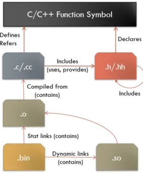
In this section first we introduce the commonly used basic terms of relationships defined between the C/C++ source files and the binary objects (see Figure 2), then present our more complex relationship definitions to describe the connections between the various kind of files in a software project at a higher abstraction level.
4.1. Preliminaries
Definition 4.1(Relations between source files). At the level of theabstract syntax tree [6], the main artifacts of a C/C++ source code are the user defined symbols2, which can be declared, defined or referred/used by either the source files (.c/.cc) or the header files (.h/.hh). A C/C++ symbol might have multiple declarations and references, but can be defined only once in a semantically correct source code.
To enforce the separation of the specification and implementation layer, header files should mainly consist of declarations, whose definitions are in the appropriate source files.3 From our perspective only those C/C++ symbols are important, which are declared in a header file and are defined or referred by a source file.
Figure 2: Relations between compilation artifacts.
2From our viewpoint only the function (and macro) symbols and their declaration, definition and usage are significant, although a similar classification for other symbol types can be established without difficulties.
3In some cases, headers may contain definition and source file may also consist forward decla- rations as an exception.
Definition 4.2(Relations between binaries). The source files of a project arecom- piled into object files, which are then statically linked into archive files (.lib/.a), shared objects or executable binaries. Shared objects are linked dynamically into the executables at runtime. To extract this information and visualize the relation- ship of binaries together with the relations declared between the C/C++ files, the analysis of the compilation procedure of the project is required beside the static analysis of the source code.
For the purpose of the presented visualization views in this paper the different kind of binary relationships is irrelevant, therefore they will be collectively referred as thecontains relation henceforward (see Figure 2).
4.2. Extended classification
The basic include relationship among the implementation and header C/C++ files have already been introduced in Section 4.1, however in order to solve the problem raised in Section 3, the definitions of the proposed uses and provides relations have to be separated.
Definition 4.3 (Provides relationship from implementation c to header h). We say that in a fileset a implementation filec provides the interface specified by the header fileh, whenc directly includeshand a common symbol sexists, for which hcontains the declaration, whilecconsists the definition of it.
Definition 4.4 (Uses relationship from implementation c to headerh). Similarly to the previous provides relationship definition, we state that in a fileset an imple- mentation file c uses the interface specified by the header file h, when c directly includes, but does not provides h and a common symbols exists, which c refers andhcontains the declaration of it.
Definition 4.5 (Interface graph (diagram) of implementation file c). Let us define a graph with the set of nodes N and set of edges E. Let P be the set of header files which areprovided bycandU the set of header files used byc, andB the set of binary files whichcontainc. We define thatN consists ofc, the elements ofP,U, andB. E consists the corresponding edges to represent the relationships between the nodes inN.
Figure 2 shows the illustration for the above mentioned definitions. Based on the idea of the Interface diagram defined in Definition 4.5, which shows the immediate provides, uses and contains relations of the examined file, we defined the following more complex file-based views.
The nodes of these diagrams are the files themselves and the edges represent the relationships between them. A labeled, directed edge is drawn between two nodes only if the corresponding files are in eitherprovides,uses orcontains relationship.
The label of the edges are the type of their relationship and they have the same direction as the relation they represent.
Definition 4.6(Used components graph(diagram) of sourcec). Let us define a graph with the set of nodes N and set of edges E, and let S be the set of implementation files which provides an interface directly or indirectly used by c.
We define thatN consists ofc, the elements ofS and the files along the path from c to the elements of S. Binaries containing any implementation file inS are also included in N. E consists the corresponding edges to represent the relationships between the nodes inN.
Intuitively we can say if sourcetis a used component ofc, thencis using some functionality defined int.
Definition 4.7 (User components graph(diagram) of sourcec). Let us define the graph with the set of nodesN and set of edgesE, and similarly to the previous definition, letS be the set of implementation files which directly or indirectlyuses the interface(s) provided by c. We define that N consists of c, the elements of S and the files along the path from c to the elements ofS. Binaries containing any implementation file inSare also included inN. Econsists the corresponding edges to represent the relationships between the nodes inN.
Intuitively we can say if sourcet is a user component ofc, thenc is providing some functionality used byt.
5. Experimental results
In order to implement the views defined in Section 4, we created a diagram visual- izing tool was created as part of a larger code comprehension supporting project – namedCodeCompass. The software is developed in cooperation at Eötvös Loránd University and Ericcson Hungary. The tool provides an interactive graph layout interface, where the users are capable of requesting more information about the nodes representing files and can also easily navigate between them, switching the perspective of the view they are analyzing.
Figure 3: Interface diagram of tinyxml.cpp.
For demonstration purposes in this paper, the open-source TinyXML parser project[10] was selected. In this section altogether three examples for the use of our tool is shown and information retrievable from them is examined.
Example 5.1. Figure 3 displays anInterface diagram, showing the immediate re- lations of a selected file with other files in the software. As the image shows, the C++ implementation file in the middle (tinyxml.cpp) includes two header files, but the special connection of implementation (provides) is distinguished from the mere uses relation. This diagram not only presents the connections between C++
source and header files, but also displays in which object file the focused imple- mentation file was compiled into through the compilation process of the project.
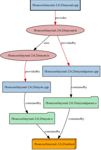
Figure 4: Used components bytinyxml.cpp.
Example 5.2. Figure 4 presents theUsed components diagram of the implemen- tation filetinyxml.cpp at the top. The goal of this visualization is to determine
which other files and compilation units the selected file depends on. As it is de- picted in the figure, the interface specification for thetinyxml.cppimplementation file is located in the tinyxml.hheader. This header file on the one part is pro- vided by thetinyxmlparser.cpp, and on the other hand uses thetinystr.h. The latter header file is provided by the tinystr.cpp source. Hence the implication can be stated that the original tinyxml.cpp indirectly uses and depends on the tinyxmlparser.cppand thetinystr.cppfile.
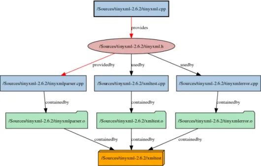
Example 5.3. Parallel to Figure 4, the following example deduces the compilation artifacts depending on the same selected source tinyxml.cpp. The User compo- nents diagram displays (see Figure 5) that this implementation file implements an interface contained by thetinyxml.hheader. This header is used or provided by three sources (tinyxmlparser.cpp,xmltest.cppandtinyxmlerror.cpp), there- fore they are the users of tinyxml.cpp.
Figure 5: User components of tinyxml.cpp.
6. Conclusions and future work
In large legacy software projects a huge codebase can easily be built up because of the extended development time, while fluctuation among programmers can also often be a significant problem. Code comprehension support addresses these ques- tions through assisting – both experienced and newcomer – developers with visu- alization views to better understand the source code. In this paper we discussed
what kind of file-level views are missing from the current code comprehension tools, regarding the relationships between different type of compilation artifacts. We de- fined our novel graph view as a solution to this problem, and demonstrated the practical use of our technique through examples on an open-source C++ project.
The new visualization techniques were found helpful and applicable for legacy soft- ware in supporting code comprehension.
Above the file-level granularity, a higher level of modularity can also be defined, considering that related files can form the interface of a reusable binary component and are often grouped together physically (i.e. contained in a directory) or virtu- ally (e.g. using packages or namespaces). Future development will generalize and expand the file-based dependency relationship definitions introduced in this paper to be applicable for modules containing multiple files.
Further work will also include the examination of how the information retrieved by our definition rules can be used in the field of architecture compliance checking.
Software systems often impose constraints upon the architectural design and im- plementation of a system, for example on how components are logically grouped, layered and how they may interact with each other. In order to keep the main- tainability of a software system through a long development time with a large programmer team, it bears extreme importance that the design and implementa- tion are compliant to its intended software architecture. Due to the complexity of large software systems, guaranteeing the compliance by manual checking is almost impossible, hence automated support is required, which is still not a completely solved issue nowadays [5].
References
[1] Balzer, M., Deussen, O., Level-of-detail visualization of clustered graph lay- outs,Proceedings of the 6th International Asia-Pacific Symposium on Visualization, (2007), 33–140.
[2] Biederman, I.,Recognition-by-components: a theory of human image understand- ing,Psychological review, Vol. 94 (1987), 115–147.
[3] Caserta, P., Zendra, O.,Visualization of the static aspects of software: a survey, IEEE Transactions on Visualization and Computer Graphics, Vol. 17 (2011), 913–
933.
[4] Gutwenger, C., Jünger, M., Klein, K., Kupke, J., Leipert, S., Mutzel, P., A new approach for visualizing UML class diagrams, Proceedings of the 2003 ACM Symposium on Software Visualization, (2003), 179–188.
[5] Pruijt, L., Koppe, C., Brinkkemper, S.,, On the accuracy of architecture com- pliance checking support: Accuracy of dependency analysis and violation reporting, IEEE 21st International Conference on Program Comprehension, (2013), 172–181.
[6] Salomaa, A.,Formal Languages,Academic Press Professional, Inc., (1987).
[7] Spence, I., Visual psychophysics of simple graphical elements,Journal of Experi- mental Psychology: Human Perception and Performance, Vol. 16 (1990), 683–692.
[8] Doxygen Tool: http://www.stack.nl/~dimitri/doxygen/.
[9] Understand Source Code Analytics & Metrics,http://www.scitools.com/.
[10] TinyXML parser,http://www.grinninglizard.com/tinyxml/.
Solving computational problems in real algebra/geometry
James H. Davenport
∗University of Bath (U.K.) J.H.Davenport@bath.ac.uk
Submitted September 16, 2014 — Accepted January 26, 2015
Abstract
We summarise some computational advances in the theory of real algebra/
geometry over the last 15 years, and list some areas for future work.
Keywords:Real algebraic geometry, cylindrical algebraic decomposition
1. Introduction
Real Algebra and Geometry have many computational applications. In theory they solve many problems of robot motion planning [34], though practice is not so kind [38]. Understanding the (real) geometry of branch cuts [16] is crucial to issues of complex function simplification [3]. A very powerful technique in computation real geometry is Cylindrical Algebraic Decomposition, introduced in [12] to solve problems of Quantifier Elimination.
Notation 1.1. We assume that the initial problem posed hasm polynomials, of degree (in each variable separately) at mostd, innvariables.
∗Thanks to Russell Bradford, Matthew England, Nicolai Vorobjov, David Wilson (Bath); Chris Brown (USNA); Scott McCallum (Macquarie); Marc Moreno Maza (UWO) and Changbo Chen (CIGIT), and to the referees. This talk grew out of an invitation to speak at ICAI 2014 in Eger, and the author is grateful to the organisers. The underlying work was supported by EPSRC grant EP/J003247/1.
http://ami.ektf.hu
35
2. Quantifier elimination
A key technique we are going to use isQuantifier Elimination: throughout,Qi ∈ {∃,∀}. Given a statement
Φ :=Qk+1xk+1. . . Qnxnφ(x1, . . . , xn),
where φ is in some (quantifier-free, generally Boolean-valued) language L, the Quantifier Elimination problem is that of producing an equivalent
Ψ :=ψ(x1, . . . , xk) : ψ∈ L. In particular,k= 0is a decision problem: isΦtrue?
The Quantifier Elimination problem is critically dependent on the languageL and the range of the variables xi. For example
∀n:n >1⇒ ∃p1∃p2(p1∈ P ∧p2∈ P ∧2n=p1+p2) [where m∈ P ≡m >1∧ ∀p∀q(m=pq⇒p= 1∨q= 1)]
is a statement of Goldbach’s conjecture in the language of the natural numbers with, naïvely, seven quantifiers (five will do if we use the same quantifiers for the two instances of P).
In fact, quantifier elimination is impossible over the natural numbers [29].
From this it follows that it is impossible over the real numbers if we allow un- restricted1 trigonometric transcendental functions in L, sincen ∈Zis equivalent to sin(nπ) = 0. The functionsinsatisfies a second-order (or coupled pair of first- order) differential equation(s), and there are positive results provided we restrict ourselves to Pfaffian functions, i.e. solutions of triangular systems of first-order partial differential equations with polynomial coefficients. Exploring this is beyond the scope of this paper: see [24].
However, quantifier elimination is possible for semi-algebraic (polynomials and inequalities)LoverR[35]. Note that we need to allow inequalities: the quantifier- free form of∃y:y2=xisx≥0, and∃y:xy= 1has the quantifier-free formx6= 0.
Formally we define the language ofreal closed fields,LRCF, to include the natural numbers, +,−,×,=, > and the Boolean operators. Then ∃y : y2 =x eliminates the quantifier to (x >0)∨(x= 0) and ∃y : xy = 1 eliminates the quantifier to (x >0)∨(0> x).
It is worth noting that in practice we nearly always treat 6= as a first-class citizen, and indeed this is necessary when proceeding via regular chains (Section 3.3).
3. Cylindrical algebraic decomposition
Unfortunately, the complexity of Tarski’s method is indescribable (in the sense that no tower of exponentials can describe it) and we had to wait for [12] for a remotely
1Note that the undecidability comes from the fact that the functionsin :R→Rhas infinitely many zeros. Restricted versions are a different matter: see [24, (h) p. 214].

![Figure 1: Division (from [13, p. 7])](https://thumb-eu.123doks.com/thumbv2/9dokorg/1206682.90135/51.722.143.581.111.543/figure-division-from-p.webp)