Annales Mathematicae et Informaticae (47.)

(1)

ANNALES

MATHEMATICAE ET INFORMATICAE

TOMUS 47. (2017)

COMMISSIO REDACTORIUM

Sándor Bácsó (Debrecen), Sonja Gorjanc (Zagreb), Tibor Gyimóthy (Szeged), Miklós Hoffmann (Eger), József Holovács (Eger), Tibor Juhász (Eger), László Kovács (Miskolc), László Kozma (Budapest), Kálmán Liptai (Eger), Florian Luca (Mexico), Giuseppe Mastroianni (Potenza), Ferenc Mátyás (Eger),

Ákos Pintér (Debrecen), Miklós Rontó (Miskolc), László Szalay (Sopron), János Sztrik (Debrecen), Gary Walsh (Ottawa)

HUNGARIA, EGER

(2)

ANNALES MATHEMATICAE ET INFORMATICAE International journal for mathematics and computer science

Referred by

Zentralblatt für Mathematik and

Mathematical Reviews

The journal of the Institute of Mathematics and Informatics of Eszterházy Károly University of Applied Sciences is open for scientific publications in mathematics and computer science, where the field of number theory, group theory, constructive and computer aided geometry as well as theoretical and practical aspects of pro- gramming languages receive particular emphasis. Methodological papers are also welcome. Papers submitted to the journal should be written in English. Only new and unpublished material can be accepted.

Authors are kindly asked to write the final form of their manuscript in L^ATEX. If you have any problems or questions, please write an e-mail to the managing editor Miklós Hoffmann: hofi@ektf.hu

The volumes are available athttp://ami.uni-eszterhazy.hu

(3)

MATHEMATICAE ET INFORMATICAE

VOLUME 47. (2017)

EDITORIAL BOARD

Sándor Bácsó (Debrecen), Sonja Gorjanc (Zagreb), Tibor Gyimóthy (Szeged), Miklós Hoffmann (Eger), József Holovács (Eger), Tibor Juhász (Eger), László Kovács (Miskolc), László Kozma (Budapest), Kálmán Liptai (Eger), Florian Luca (Mexico), Giuseppe Mastroianni (Potenza), Ferenc Mátyás (Eger),

Ákos Pintér (Debrecen), Miklós Rontó (Miskolc), László Szalay (Sopron), János Sztrik (Debrecen), Gary Walsh (Ottawa)

INSTITUTE OF MATHEMATICS AND INFORMATICS ESZTERHÁZY KÁROLY UNIVERSITY OF APPLIED SCIENCES

HUNGARY, EGER

(4)

HU ISSN 1787-6117 (Online)

A kiadásért felelős az Eszterházy Károly Egyetem rektora Megjelent a Líceum Kiadó gondozásában

Kiadóvezető: Nagy Andor Felelős szerkesztő: Zimányi Árpád Műszaki szerkesztő: Tómács Tibor Megjelent: 2017. december Példányszám: 30

Készítette az

Eszterházy Károly Egyetem nyomdája Felelős vezető: Kérészy László

(5)

Steganalysis of digital contents, based on the analysis of unique color triplets

Anna Akhmametieva

Department of Informatics and Management of Information Systems Security, Odessa National Polytechnic University, Ukraine

anna-odessitka@mail.ru

Submitted June 24, 2016 — Accepted December 22, 2016

Abstract

The new steganalytic algorithm for detection of the presence of additional information that embeds into digital images and digital videos by LSB Match- ing method with a small hidden capacity (not more than 0.5 bpp) is presented.

The proposed steganalytic algorithm analyses digital content in the spatial domain and is based on the accounting of sequential color triads in the matrix of unique colors of the digital content. Steganalytic algorithm has a high effectiveness of detecting the additional information embedded into one arbitrary color component of the container with a small hidden capacity.

Keywords:Steganalysis, LSB Matching, the spatial domain of the container, a digital image, a digital video

MSC:68U10, 94A08, 68P30

1. Introduction

The rapid development of information and communication technologies leads to their wide distribution in the state, public and household sectors, it is possible easily and quickly to transfer any information to long distances. If in the state activities secure channels of communication applies, then such open channels as e-mail, social networks allows to exchange externally innocuous data, therefore they are often used with criminal intentions. Open access to the Internet and scientific resources allows you to track newest developments in the field of information security, steganography and steganalysis. The use of steganographic methods

http://ami.uni-eszterhazy.hu

3

(6)

and algorithms allows to transfer confidential information via open communication channels by hiding the fact of its presence in the transmitted content. In a competitive environment, in the conditions of the spread of terrorism the hidden communication can lead to significant losses for businesses and to the catastrophic consequences of terrorist attacks for the society in general.

To prevent the criminal acts with using steganography it is extremely important to develop steganalysis aimed at the detecting the fact of the presence/absence of hidden information in any digital content (see [1]). Digital images, audio or video sequences can be used as containers in steganography.

Ones of the most widespread steganographic methods are different variations of the method of modification of the least significant bit (LSB Matching, LSB Replace- ment etc.) due to the simplicity of realization and the possibility of its use both in the spatial domain and in the transformation domain. Nevertheless, continuous improvement of steganographic developments impedes using of LSB method with a high hidden capacity, because it is easy to detect such embedding. Therefore, to ensure concealing of the secret communication LSB method is often used with a small hidden capacity (less than 0.5 bpp), which greatly complicates the process of detecting the presence/absence of the additional information.

A large number of steganalysis developments aimed at the detection of the presence/absence of additional information, embedded by LSB Matching method into digital images. There are enough effective steganalysis methods and algorithms (see [2, 3, 4, 5, 6, 7, 8]), that analyse digital images in the transformation domain (frequency domain, the singular/spectral decompositions of the corresponding matrices, etc.), however transfer of a digital content to transformation domain and back leads to the additional accumulation of computational errors, which consid- erably complicates the process of detecting presence of additional information that embeds with a small hidden capacity.

The steganalytic methods that analyse spatial domain of digital contents allows to avoid both additional time expenses, and accumulation of computational errors, however existing developments (see [9, 10, 11, 12, 13]) often have low effectiveness when embedding of additional information is carried out by LSB Matching method with a small hidden capacity.

The use of a digital video as a container in steganography allows to transfer a significant amount of data due to the large number of frames, using at the same time a small hidden capacity. It is very problematic to detect the presence of additional information in these conditions. However, despite advantages of using of digital videos, in open access there are not a lot of works devoted to video steganalysis. Widely spread are methods that analyses spatial (see [14]) and temporal (see [15, 16]) domains of digital video, as well as specialized methods directed against steganographic tools such as embedding of additional information to the motion vectors (see [17]) or H.264/AVC (see [18]).

Taking into account the advantages of steganalysis in the spatial domain, the aim is to develop steganalytic algorithm aimed to detect embedding of additional information by LSB Matching with a small hidden capacity (no more than 0.5 bpp)

(7)

into digital containers, which are color digital images and digital videos.

2. Research essence

As containers we consider color digital images and digital videos stored according to the RGB color scheme. We will use term "cover" (cover-image or cover-video) for the unfilled containers. Each video sequenceV consists of framesFl(m, n), where l = 1, K, K - number of frames, m - frame height, n - frame width. Additional information, which is a binary sequence, embeds by LSB Matching into the spatial domain of the randomly selected color component of the container. Result of embedding of additional information to the container we will call stego (stego- image or stego-video). It should be noted that if as a container the image in a losses format is used, it will be resaved in a lossless format after embedding of additional information.

LSB Matching method is realized according to the formula (see [10]):

ps(i, j) =





pc(i, j) + 1 ifb6=LSB(pc(i, j))&r >0, pc(i, j) ifb=LSB(pc(i, j)),

pc(i, j)−1 ifb6=LSB(pc(i, j))&r <0, (2.1) wherepc(i, j),ps(i, j)- the brightness value of the pixel of the color matrix of the original digital image/frame and stego respectively, b - bit of the secret message, r - a random value in the range [−1,+1] , LSB(p) - the least significant bit of p (see [10]). Thus, embedding of additional information or will increase pixel’s brightness value of an original matrix on 1 (+1), or will reduce it on 1 (−1), or will remain it unchangeable (0).

Each frame of the video sequenceV is an image formed by three color components: red, green and blue matrices of sizem×n. Accordingly, each pixel of the frame/image is represented as a triplet of values(R, G, B). All triplets(ri, gi, bi), i = 1, k, k = m·n, that occur in a digital image/frame of a digital video form some matrix CT (color triplets) of size k×3. Triplets can repeat in the matrix CT, depending on that how often they appear in a digital image/frame of a digital video.

Definition 2.1. All of the triplet’s various values (R, G, B) we will call unique colors, their number is denoted byU.

Definition 2.2. A matrix of sizeU×3of ordered unique colors(rj, gj, bj),j= 1, U we will call the matrix of unique colorsU CT (unique color triplets).

The matrix of unique colors in MathWorks MatLAB can be received by standard procedure U CT =unique(CT,⁰rows⁰), where parameter ⁰rows⁰ denotes that the matrix U CT will contain unique rows (triplets) of matrixCT. Thus, the matrix U CT is an ordered sequence of unique colors which at least once occur in the analyzed digital image/frame of a digital video. The matrix of unique colors does

(8)

not take into account the frequency of appearance of some triplet(R, G, B)⊂U CT in the container.

Consider what changes the matrix of unique colors will be undergone when additional information embeds to the container by LSB Matching according to the formula 2.1.

Let to some pixel of the container (for example, a digital image) forming the triplet (95,116,68) additional information embeds into a green color component.

This triplet will be included in the matrix of unique colors of the container as it at least once occurs in the digital image. Embedding of the bit of information into a green color component of the pixel can change it value or on (95,115,68), or on (95,117,68), or to leave it without change. Let the pixel value will take (95,117,68). If the triplet is founded in the digital image only once, then matrix of unique colors of stego after embedding of additional information will not contain original triplet(95,116,68), but its modification(95,117,68)will appear. However, many different pixels in the container can have the same color, i.e. the triplet occurs in the container as a rule repeatedly. Therefore, after embedding of additional information into different pixels of the same color, they can be modified by all three ways: +1,−1,0, that will lead to appearance of all three modifications of triplets in the matrix of unique colors of stego (in this example, (95,115,68),(95,116,68) and(95,117,68)).

Similar modifications occur when additional information embeds into red or blue color components.

Thus, in case of embedding of additional information into container in the matrix of unique colors there will be additional triplets differing from original on

±1in that color component where embedding was carried out.

Introduce the following definitions.

Definition 2.3. Under a sequential Red-triad for the current triplet(rj, gj, bj),j= 1, U, in the matrix of unique colors we will understand execution of the condition:

(rj, gj, bj)⊂U CT AND(rj−1, gj, bj)⊂U CT AND(rj+ 1, gj, bj)⊂U CT, j= 1, U.

The Red-triad corresponds to the red color component of the container.

Definition 2.4. Under a sequential Green-triad for the current triplet(rj, gj, bj), j= 1, U, in the matrix of unique colors we will understand execution of the condition:

(rj, gj, bj)⊂U CT AND(rj, gj−1, bj)⊂U CT AND(rj, gj+ 1, bj)⊂U CT, j= 1, U.

The Green-triad corresponds to the green color component of the container.

Definition 2.5. Under a sequential Blue-triad for the current triplet (rj, gj, bj), j= 1, U, in the matrix of unique colors we will understand execution of the condition:

(9)

(rj, gj, bj)⊂U CT AND(rj, gj, bj−1)⊂U CT AND(rj, gj, bj+ 1)⊂U CT, j= 1, U.

The Blue-triad corresponds to the blue color component of the container.

Definition 2.6. The basic triad is a sequential triad corresponding to that color component of the container, into which embedding of additional information was carried out.

Definition 2.7. Concomitant triads are that sequential triads that corresponds to unfilled color components of the container.

I.e. after embedding of additional information into blue color component the basic triad is Blue-triad and concomitant triads are Red- and Green-triads.

The computational experiment that analyses the quantity of Red-, Green- and Blue-triads in unfilled digital containers was carried out.

There are the following digital images as containers:

1. Set 1: 203 color digital images from [19] in JPG format;

2. Set 2: 201 high-quality digital images from [20] in JPG format;

3. Set 3: 215 images received by non-professional photo cameras in JPG format;

4. Set 4: 200 color digital images from [19] in TIFF format;

5. Set 5: 200 images received by non-professional photo cameras in TIFF format.

The quantity of sequential triads in the matrix of unique colors of unfilled digital containers stored in losses format (Set 1, 2, 3) does not exceed 3% of total number of unique colors, unlike containers stored in lossless format (Set 4, 5) where even in the absence of additional information the quantity of Red-, Green- and Blue-triads reaches 40-60% due to the lack of compression and, consequently, a large variety of unique colors. At the same time it is noted that the relative quantity of Red-, Green- and Blue-triads (relative to the number of unique colors) in unfilled digital images is comparable by values, i.e. the difference is not more than 1-1.5%.

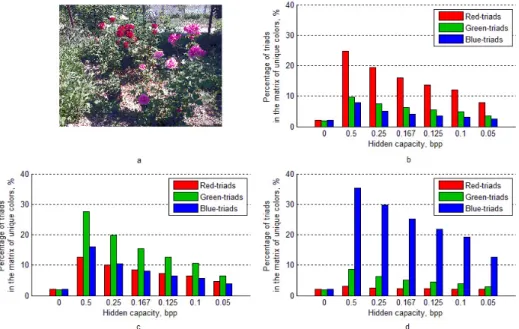
Analyze how the number of sequential triads in the matrix of unique colors will change when additional information embeds into one arbitrary color component of the container with different values of hidden capacity. Consider as a container the digital image in losses format (Figure 1, a), into which additional information is embedded into a red color component by LSB Matching with different values of hidden capacity. Counting of Red-, Green- and Blue-triads in the matrix of unique colors of the formed stego was carried out. Counting of each kind of sequential triads dictated by the fact that in the process of steganalysis it is unknown, into what kind of color components additional information has been embedded. The percentage of Red-, Green- and Blue-triads in relation to the total number of unique colors of stego formed by embedding of additional information to the red color component with different values of hidden capacity is shown in Figure 1, b. Similarly,

(10)

the quantity of Red-, Green- and Blue-triads in matrices of unique colors of stegos formed by embedding of additional information only into green color component (Figure 1, c) and only into blue color component (Figure 1, d) is determined.

Figure 1: The quantity of sequential color triads in the image stored in losses format: a – original digital image from Set 3; b - percentage of sequential triads in the stego formed by embedding of additional information by LSB Matching into red color component; c - percentage of sequential triads in the stego formed by embedding of additional information by LSB Matching into green color component; d - percentage of sequential triads in the stego formed by embedding of additional information by LSB Matching into blue

color component

As can be seen from Figure 1, embedding of additional information into one arbitrary color component causes a significant increase in the quantity of basic triads. At the same time the number of concomitant triads increases too, however less in comparison with the quantity of basic triads in the matrix of unique color of stego. This growth is associated with an increase in the number of unique colors when additional information has been embedded and is random. For example, embedding of additional information into blue color component leads to change of unique triplet(10,158,74)on Blue-triad(10,158,73),(10,158,74)and(10,158,75).

If there are triplets(11,158,75)and(12,158,75)in the matrix of unique colors of stego then they with a new triplet(10,158,75)forms Red-triad, but embedding of additional information into red color component has not performed.

(11)

If as the container to use the image in lossless format then embedding of additional information practically does not influence the percentage of consecutive triads, what is shown in Figure 2, where into image in a lossless format (Fig- ure 2, a) additional information embeds into a red color component (for example), the percentage of Red-, Green- and Blue-triads for which is shown in Figure 2, b.

The similar situation is observed when additional information embeds into another color component and is typical for all digital images in a lossless format. Thus, further as containers only digital contents in losses format will consider.

Figure 2: The quantity of sequential color triads in the image stored in lossless format: a – original digital image from Set 4; b - percentage of sequential triads in the stego formed by embedding of additional information by LSB Matching into red color component

Figure 1 shows that the percentage of concomitant triads in the matrix of unique colors of stego increases on average up to 8-12%. Accept preliminary thresholds of the quantity of sequential triads Tlow = 2.5 and Tup = 8 for detection of the presence/absence of additional information in the digital content. On the basis of digital images from the Set 1, 2, 3 the computational experiment, determining percentage of Red-, Green- and Blue-triads in matrices of unique colors of original containers (hidden capacity 0 bpp) and stegos formed by embedding of additional information only into one arbitrary color component with different values of hidden capacity was carried out. Results of the experiment are shown in Table 1, where pc – the quantity (in %) of all sequential triads (and basic, and concomitant) in matrices of unique colors of digital contents,max(pc)- maximum percentage of sequential triads in matrices of unique colors of digital contents (for hidden capacity 0.05-0.5 bpp max(pc) corresponds to the maximum containing of basic triads in stego sets).

Thus, the computational experiment showed that an average of 90% of digital containers stored in losses format, contain no more than 2.5% Red-, Green- and Blue-triads, their number significantly increases after embedding of additional information. Therefore, the condition for the original container is performance of the relationship:

(12)

Set Threshold Hidden capacity, pbb

0.5 0.25 0.167 0.125 0.1 0.05 0

Set 1 pc≤Tlow 3.61 6.24 8.21 8.70 9.20 13.30 94.42 pc > Tup 89.66 80.79 72.58 64.37 56.49 35.80 0.33 max(pc) 56.94 47.44 47.68 45.33 43.22 31.36 9.08 Set 2 pc≤Tlow 3.15 5.31 6.30 8.62 11.61 18.24 86.24

pc > Tup 84.25 69.98 64.18 55.89 53.57 31.01 0.83 max(pc) 54.58 51.67 48.76 46.21 41.47 36.02 11.25 Set 3 pc≤Tlow 1.40 4.65 5.89 6.82 7.60 9.92 92.25

pc > Tup 90.70 85.74 77.36 68.22 61.24 46.98 0 max(pc) 55.08 51.65 48.28 45.32 43.80 38.53 4.69 Table 1: The percentage of sequential triads in the matrix of unique

colors of digital images

(pR≤Tlow)AND(pG≤Tlow)AND(pB≤Tlow), and back again for stego:

(pR > Tlow)OR(pG > Tlow)OR(pB > Tlow),

where Tlow = 2.5, pR- the percentage of Red-triads in the matrix of unique colors, pG - the percentage of Green-triads in the matrix of unique colors, pB - the percentage of Blue-triads in the matrix of unique colors.

ThresholdTup = 8promotes to correctly detection of unfilled containers, providing the protection against the appearance of "false alarms".

Based on the established features of the changes in the number of color triads in the matrix of unique colors the steganalytic algorithm for detecting embedding of additional information by LSB Matching into spatial domain of digital containers (digital images and digital videos) is proposed. If digital images are as containers, it is necessary only first step of the algorithm for detecting.

2.1. Designations employed in the algorithm

Fl(m, n), l= 1, K - frame of the analyzed video sequenceV consisting ofK frames of size m×n.

resultF - a matrix of sizeK×3, containing the result of the detection on each frame of the video sequence (sequence of digital images). In the case of a single digital image the matrixresultF is a matrix of size 1×3 and is the end result of the detection. The first column of the matrix corresponds to red color component, the second – to green color component, and the third - to blue color component.

Value 1 of the matrix corresponds to the presence of additional information in the corresponding color component, 0 - to its absence.

U CT - a matrix of unique colors of the frame Fl (image I) of size U ×3, containing unique triplets(rj, gj, bj), j= 1, U.

(13)

countR, countG, countB - number of sequential triads in the U CT for red, green and blue color components, respectively.

pR, pG, pB - percentage of sequential triads in the U CT in relation to total number of unique colors for red, green, blue color components, respectively.

kRpos,kGpos,kBpos - number of positive definite frames as containing embedded additional information in red, green and blue color components of the frame, respectively.

kRneg, kGneg, kBneg - number of negative definite frames as not containing embedded additional information in red, green and blue color components of the frame, respectively.

2.2. Steganalytic algorithm

Step 1(for digital images and frames of video sequence). For each imageI(frame Fl, l= 1, K) the detection of the presence of additional information performs.

1. Forming of the matrix of unique colorsU CT of the digital image I / frame Fl of video sequenceV.

2. Counting of Red-, Green-, Blue-triads.

(a) If for the current triplet (rj, gj, bj), j = 1, U in the U CT at the same time there are triplets(rj+ 1, gj, bj)and(rj−1, gj, bj)thencountR= countR+ 1;

(b) If for the current triplet (rj, gj, bj), j = 1, U in the U CT at the same time there are triplets(rj, gj+ 1, bj)and(rj, gj−1, bj)thencountG= countG+ 1;

(c) If for the current triplet (rj, gj, bj), j = 1, U in the U CT at the same time there are triplets(rj, gj, bj+ 1)and(rj, gj, bj−1)thencountB= countB+ 1.

3. To compute:

pR= countR

U ·100,pG=countG

U ·100,pB=countB U ·100.

4. Detection of the presence/absence of additional information in the digital imageI / single frameFl,l= 1, K, of video sequenceV.

(a) if(pR=max(pR, pG, pB))AND(pR > Tup) thenresultFl,1= 1,

else if

(pR > Tlow ORpG > Tlow ORpB > Tlow) AND (pR >1.5·pG AND pR >1.5·pB)

thenresultFl,1= 1, elseresultFl,1= 0;

(14)

(b) if(pG=max(pR, pG, pB))AND(pG > Tup) thenresultFl,2= 1,

else if

(pR > Tlow ORpG > Tlow ORpB > Tlow) AND (pG >1.5·pRAND pG >1.5·pB)

thenresultFl,2= 1, elseresultFl,2= 0;

(c) if(pB=max(pR, pG, pB))AND(pB > Tup) thenresultFl,3= 1,

else if

(pR > Tlow ORpG > Tlow ORpB > Tlow) AND (pB >1.5·pRAND pB >1.5·pG)

thenresultFl,3= 1, elseresultFl,3= 0.

Step 2 (for video sequences). Counting of positive and negative detection results in frames of a video sequence separately for each color component in the matrixresultF:

1. ifresultFl,1= 1

thenkRpos=kRpos+ 1, elsekRneg=kRneg+ 1;

2. ifresultFl,2= 1

thenkGpos=kGpos+ 1, elsekGneg=kGneg+ 1; 3. ifresultFl,3= 1

thenkBpos=kBpos+ 1, elsekBneg=kBneg+ 1.

Step 3(for video sequences). Detection of the presence/absence of additional information in a digital video:

1. ifkRpos≥kRneg

then additional information contains in a red color component, else additional information is absent in a red color component;

2. ifkGpos≥kGneg

then additional information contains in a green color component, else additional information is absent in a green color component;

3. ifkBpos≥kBneg

then additional information contains in a blue color component, else additional information is absent in a blue color component.

(15)

3. Results of the experiment

In the computational experiment aimed at verifying the work of the proposed steganalytic algorithm, digital contents from the Set 1, 2, 3 and 367 video sequences of frame size 320×240 obtained by the mobile cameras (Set V) have been used.

Each video contains in average 250 frames.

It should be noted that color photos and videos obtained by the cameras of mobile devices (Set 3 and Set V) are the most probable containers as the most widespread due to permanent presence smart phones, IPad or other mobile devices with itself. Original mobile videos are stored in a losses format and has the extension *.3gp or *.mp4. After embedding of additional information video are saved as uncompressed video in *.avi format.

Embedding of additional information was carried out into a randomly selected color component of digital images and videos with different values of hidden capacity: 0.5 bpp, 0.25 bpp, 0.167 bpp, 0.125 bpp, 0.1 bpp, 0.05 bpp. When additional information embeds into video sequence the selected color component is constant for all frames. Such embedding is caused by the fact that, as a rule, in case of steganography data transmission one component is used as the container and its choice is part of the secret key.

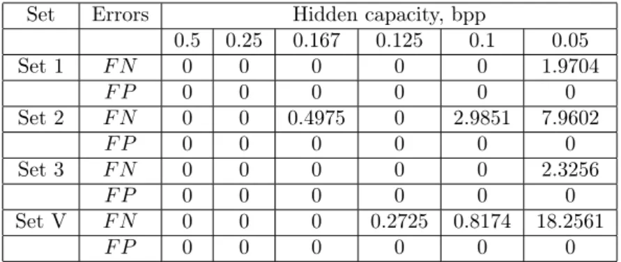
By results of experiment type I errors (False NegativeF N) – the pass stego in case of its presence and type II errors (False Positive F P) – false detection stego in case of its absence (Table 2) were received.

Set Errors Hidden capacity, bpp

0.5 0.25 0.167 0.125 0.1 0.05

Set 1 F N 0 0 0 0 0 1.9704

F P 0 0 0 0 0 0

Set 2 F N 0 0 0.4975 0 2.9851 7.9602

F P 0 0 0 0 0 0

Set 3 F N 0 0 0 0 0 2.3256

F P 0 0 0 0 0 0

Set V F N 0 0 0 0.2725 0.8174 18.2561

F P 0 0 0 0 0 0

Table 2: The effectiveness of detecting the presence/absence of additional information in digital contents, %

Table 2 shows that errors in detecting the presence of embedding of additional information in a digital content are very small, even for hidden capacity 0.05 bpp, indicating the high effectiveness of the proposed steganalytic algorithm.

For comparing of the effectiveness of the developed steganalytic algorithm with other existing methods for detection of embedding of additional information by LSB Matching in digital images stored in a losses format, the ROC-analysis is used.

(16)

ROC-curve analysis method applied to the steganalysis lies in realization of the testing of the group of digital images, that includes both unfilled containers, and stego, and it is known what each image is. Among analyzed digital images in a test group it is necessary to identify the stego (classV1) and original containers (class V2) using the developed steganalytic algorithm, as a result of which a positiveδ= 1 (stego) or negativeδ= 0(cover) decision is adopted. Test results can be presented as Table 3 (see [3]), where T P is the quantity of correctly identified stego,T N is the quantity of correctly identified unfilled containers.

True state of digital image Result of detection δ= 1- stego δ= 0 - cover

classV1- stego T P F N

classV2- cover F P T N

Table 3: Results of detection of the test group of digital images

Obtained detection results are presented in the two-dimensional ROC-space, where the X-axis represents the specificity values that characterize the type II errors:

Sp= T N T N+F P,

and the Y-axis represents the sensitivity, characterizing the type I errors:

Se= T P T P +F N.

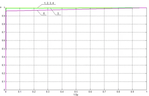
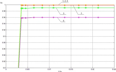
In this study values Sp and Se are defined for different values of parameter Tlow, based on which ROC-curves for values of hidden capacity 0.5, 0.25, 0.167, 0.125, 0.1 and 0.05 bpp shown in Figure 3, 4 are constructed. Figure 3 shows the ROC-space in the range 1−Sp ⊂0,1, Se ⊂0,1, Figure 4 shows a fragment of ROC-space in the range1−Sp⊂0,0.025,Se⊂0.8,1.

Based on the constructed ROC-curves an integral parameter ρ characterizing the effectiveness of the studied steganalytic algorithm is obtained, whereρ= 2A−1, A - the area under the ROC-curve. The values of area A and parameter ρ for different values of hidden capacity are given in Table 4.

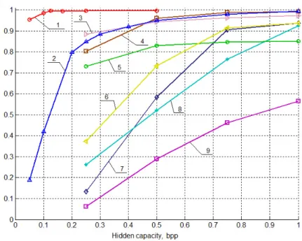
Comparison of the effectiveness of the steganalytic algorithm based on the analysis of color triads with other modern analogues for digital images (Ker’s (see [7]), Liu’s (see [8]), HGE, NDH COM, RLH COM, Fused feature, Joint feature set (see [9]), SAVV (see [3])) is carried out by comparing the integral parameters ρ for the corresponding values of hidden capacity. Visual comparison of the above methods is shown in Figure 5 (see [3]).

As can be seen from Figure 5, the results of detecting the presence/absence of embedding of additional information by LSB Matching in digital images are far superior previous solutions (see [3, 7, 8, 9]), especially in the case of a small hidden capacity (0.25 bpp or less). The most revealing is the comparison of the

(17)

Figure 3: ROC-curves that characterizes the work of the steganalytic algorithm for detection of the presence of additional information embedded by LSB Matching into digital images with different values of hidden capacity: 1 - 0.5 bpp; 2 - 0.25 bpp; 3 - 0.167 bpp;

4 - 0.125 bpp; 5 - 0.1 bpp; 6 - 0.05 bpp

Hidden capacity, bpp A ρ

0.5 0.99822294 0.99644588

0.25 0.99822294 0.99644588

0.167 0.997393263 0.994786526 0.125 0.99822294 0.99644588

0.1 0.993238873 0.986477747 0.05 0.977475004 0.954950008 Table 4: Values of the integral parameterρfor evaluating the effectiveness of the steganalytic algorithm for detection of the presence

of additional information embedded by LSB Matching

developed algorithm with method SAVV, analyzing digital images with a small hidden capacity.

In modern papers devoted to steganalysis of digital videos [14-17] in computational experiments the methods of embedding of additional information that are different from LSB Matching, are used, that does not allow correctly to compare the effectiveness of the algorithm based on the accounting of color triads in the matrix of unique colors with other analogues. However, as seen from results of the computational experiment (Table 2, set V), the developed steganalytic algorithm

(18)

Figure 4: Fragment of ROC-curves in the ROC-space in the range 1−Sp ⊂0,0.025, Se ⊂0.8,1 that characterizes the work of the steganalytic algorithm for detection of the presence of additional information embedded by LSB Matching into digital images with different values of hidden capacity: 1 - 0.5 bpp; 2 - 0.25 bpp; 3 -

0.167 bpp; 4 - 0.125 bpp; 5 - 0.1 bpp; 6 - 0.05 bpp

is effective also in case of detection of the presence/absence of additional information in digital video sequences, at the same time both the frame analysis, and the analysis of digital video as a whole are possible.

4. Conclusions

In this paper a new steganalytic algorithm of detection of the presence/absence of additional information embedded by LSB Matching with a small hidden capacity (no more than 0.5 bpp) into one color component of digital images and digital videos stored in losses formats is proposed.

Comparison of the developed steganalytic algorithm with other modern tools of steganalysis showed that the algorithm based on the accounting of color triads in the matrix of unique colors is more effective than analogues, including for very small values of hidden capacity (0.1 and 0.05 bpp). The high effectiveness of the proposed algorithm for small values of hidden capacity is provided by its work in the spatial domain of digital contents, and as a result, there are no additional computational errors.

The proposed algorithm carries out an analysis of digital images and digital

(19)

Figure 5: The results of comparing the effectiveness of the work of the steganalytic algorithm Color Triads with existing analogs for the detection of digital images: 1 - Color Triads, 2 - SAVV, 3 - Joint feature set, 4 - Liu’s, 5 - RLH COM, 6 - Fused feature, 7 - Ker’s, 8

- NDH COM, 9 – HGE

videos, for which its use can be expanded by analysis of single frames in the video sequence if additional information embeds not into all frames, but only into a small part of the total number of frames.

References

[1] Bohme, R., Advanced statistical steganalysis, Springer, 2010.

[2] Bobok, I.I., Steganalytic method for the digital signal-container stored in a losses format,Modern Information Security, Vol. 2 (2011), 50–60.

[3] Bobok, I.I., Application of ROC-analysis for integrated assessment of steganalysis method’s efficiency, Informatics and Mathematical Methods in Simulation, Vol. 2, No. 3 (2012), 221–230.

[4] Alimoradi, D., The effect of correlogram properties on blind steganalysis in JPEG images,Journal of computing and security, Vol. 1, No. 1 (2014), 39–46.

[5] Visavalia, S.R., Ganatra A., Improving blind image steganalysis using genetic algorithm and fusion technique,Journal of computer science, Vol. 1 (2014), 40–46.

(20)

[6] Yamini, B., Sabitha R., Blind steganalysis: to analyse the detection rate of stego images using different steganalytic techniques with support vector machine classifier, International journal of computer applications, No. 2 (2014), 22–25.

[7] Ker, A.D., Steganalysis of LSB matching in grayscale images, IEEE Signal Pro- cessing Letters, Vol. 12, No. 6 (2005), 441–444.

[8] Liu, Q.Z., Sung A.H., Image complexity and feature mining for steganalysis of least significant bit matching steganography, Information Sciences, Vol. 178, No. 1 (2008), 21–36.

[9] Zhihua Xia, Lincong Yang, A Learning-Based Steganalytic Method against LSB Matching Steganography,Radioengineering, Vol. 20, No. 1 (2011), 102–109.

[10] Jun Zhang, Yuping Hu, Zhibin Yuan, Detection of LSB Matching steganography using the envelope of histogram,Journal of computers, Vol. 4, No. 7 (2009), 646–653.

[11] Geetha, S., Sindhu S., Kamaraj N., Close color pair signature ensemble adaptive threshold based steganalysis for LSB embedding in digital images,Transactions on Data Privacy, Vol. 1, Iss. 3 (2008), 140–161.

[12] Mitra, S., Roy T., Mazumdar D., Saha A.B., Steganalysis of LSB Encoding in Uncompressed Images by Close Color Pair Analysis,IIT Kanpur Hackers’ Workshop 2004 (IITKHACK04), 23-24 Feb 2004, 23–24.

[13] Rudnitskiy, V., Uzun, I., Steganalysis algorithm for images that have been lossy compressed,Information Security, Vol. 15, No. 2 (2013), 122–127.

[14] Xikai Xu, Jing Dong, Tieniu Tan, Universal spatial feature set for video steganalysis,Image Processing (ICIP), 19th IEEE International Conference, Sept. 30 - Oct. 3 2012, 245–248.

[15] Pankajakshan, V., Ho, A.T.S., Improving video steganalysis using temporal cor- relation,3rd International Conference on Intelligent Information Hiding and Multi- media Signal Processing, 26-28 Nov 2007, Kaohsiung, TAIWAN.

[16] Budhia, U., Kundur, D., Zourntos, T., Digital video Steganalysis exploiting Statistical Visibility in the Temporal domain, IEEE Transactions on Information Forensics and Security, Vol. 1, Iss. 4 (2006), 502–516.

[17] Tasdemir, K., Kurugollu, F., Sezer, S., Video steganalysis of LSB based motion vector steganography, Visual Information Processing (EUVIP), 4th European Workshop, 10-12 June 2013, 260–264.

[18] Songbin Li, Peng Liu, Qiongxing Dai, Xiuhua Ma, Haojiang Deng, Detec- tion of Information Hiding by Modulating Intra Prediction Modes in H.264/AVC, Proceedings of the 2nd International Conference on Computer Science and Electron- ics Engineering (ICCSEE), 2013, 590-593.

[19] NRCS Photo Gallery. Online: http://photogallery.nrcs.usda.gov.

[20] WallpapersCraft. Online: http://wallpaperscraft.ru/.

(21)

First derivatives of fuzzy surfaces

Jan Caha

^a

, Jiří Dvorský

^b

aDepartment of Regional Development and Public Administration, Mendel University in Brno, Zemědělská 1, 613 00, Brno, Czech Republic

jan.caha@mendelu.cz

bDepartment of Computer Science,VŠB - Technical University of Ostrava, 17. listopadu 15, 708 33 Ostrava-Poruba, Czech Republic

jiri.dvorsky@vsb.cz

Submitted October 10, 2016 — Accepted July 25, 2017

Abstract

The presented research shows how the first derivatives (slope and aspect) can be calculated from a fuzzy surface by the means of fuzzy arithmetic within the geographic information system. The proposed method works with fuzzy numbers of arbitrary shape which helps with more precise specification of input values as well as more exact calculation of results. Three most important methods of partial derivatives calculation based on finite elements approximation of a surface are presented and discussed. The presented approach provides an alternative for uncertainty propagation that is commonly performed by the utilization of statistics and the Monte Carlo method in geographic applications. The example calculation shows the differences between the obtained results calculated with the utilization of fuzzy arithmetic and the Monte Carlo method.

Keywords: fuzzy surface, fuzzy arithmetic, surface derivatives, uncertainty propagation

MSC:03B52, 26E50, 90C70

1. Introduction

The process of modelling surface from a finite set of samples is a common problem in geosciences. Surfaces are often treated as certain and error-free models [41]

even though there is a wide set of reasons why they are not. Perhaps the biggest

http://ami.uni-eszterhazy.hu

19

(22)

issue arises from incomplete knowledge about the surface under study [32]. A user cannot be sure that the sample of surface values contains values that are representative enough to construct a precise surface. There is also the issue of measurement precision of the individual sample point, some authors point out that every measurement is fuzzy, at least to some extent, because there are no absolutely precise measurements [26, 37]. Another uncertainty can be introduced to the surface by the selection of interpolation technique [32]. Not only there is a range of methods that can be used for interpolation (IDW, spline interpolators, kriging etc.) but some of these methods have parameters (e.q. tension of spline, parameters of variogram in kriging) containing epistemic uncertainty. The values of these parameters are selected by the user and their selection is partially arbitrary [27]. In fact, these parameters are better described as a set of possible values than a single value which may not be correct. Authors [25] argue that much, if not the most, of uncertainty of surfaces in geosciences is interval, fuzzy or possibilistic in its nature. Fisher [13] mentions that the fuzzy set theory should be used if the definition of a class or an individual object is vague. The individual object in the case of a surface, represented commonly in geographic information system (GIS) by a grid, is a cell and its value is definitely vague because it can be based on uncertain data, influenced by epistemic uncertainty in the interpolation method [27] and even the grid model itself is a simplification and idealization of a real surface, which introduces yet another source of uncertainty [11].

Based on these facts a model of surface that would account for its inherent uncertainty is needed [26]. Such model was firstly proposed in [8] and [4]. A fuzzy surface as described in [8] is a result of interpolation with imprecise data, while the model in [4] was based on precise data but imprecise variogram in kriging interpolation. These two studies were the first to introduce fuzzy numbers into spatial modelling and spatial prediction but the applications of fuzzy approaches for predictions and modelling were used in mathematics before [36]. Later, more techniques and approaches for the construction of fuzzy surfaces emerged, including bayesian fuzzy kriging [3], kriging with imprecise variograms was further improved [27], the inverse-distance weighting method [37], and spline interpolators [2, 26, 32].

The definition of a fuzzy surface is only slightly different from an ordinary surface. A fuzzy surface is described by a set of points with knownx, y coordinates and a fuzzy numberZ˜that represents the possible values ofzat this location. The fuzzy number that describes such set of possible values represents the vague, imprecise or ill-know value. However, this uncertainty of the value does not originate in variability [25]. Similar deduction was done in [30], who mentions that statistical models often require more information about uncertainty than a user actually has. In such situations it might be reasonable and useful to formalize uncertainty in an alternative way which could be amongst others by the usage of the fuzzy set theory. Since methods for the creation of a fuzzy surface are either based on interpolation with imprecise input data, imprecise parameters of the interpolation and rarely on other methods, the outcome naturally contains this uncertainty. In- stead of storing only one value of elevation at any point of the surface, the fuzzy

(23)

surface stores a range of possible values (Fig. 1) that the surface can have at the given point. Fuzzy surfaces are an alternative to probabilistic surfaces that are commonly used in geography to estimate the influence of uncertainty on surface analyses [20, 31, 41]. While both these approaches have a lot in common there are also fundamental differences regarding the way how the resulting uncertainty is calculated and also about semantics of the results [30].

x z y

Figure 1: 3D visualization of a small fuzzy surface

The statistical approach to surface uncertainty tries to conceptualize uncertainty that occurs within the whole area of the surface through the specification of its spatial autocorrelation parameters [31]. The most commonly used method for statistical processing of uncertainty within GIS field is the Monte Carlo method [20]. Fuzzy surfaces are focused mainly on modelling uncertainty of a single cell in a grid [1, 25] while not accounting for the spatial autocorrelation explicitly. However, when the spatial autocorrelation of uncertainty is considered, it requires the user to describe it very precisely, by the specification of parameters of the autocorrelation function. This information is very rarely available to the user [30] which leads to providing of expert estimates instead of exact values [31].

As noted in [14], fuzzy mathematics has been rarely employed to actually analyse fuzzy surfaces, even though fuzzy surface exist ín geosciences for a long time.

However, some examples of calculations of fuzzy slopes [6, 16, 37] and the visibility analysis on fuzzy surfaces [1] exist. All of them are, however, rather a cases of specific examples that describes only one method with specific type of fuzzy surface. In this article we summarize several methods for the calculation of slope and aspect from the fuzzy surfaces that are working with the arbitrary type of fuzzy numbers. The presented methods should provide an approach for the fuzzy slope and the fuzzy aspect calculation as general as possible. Further the presented method serves as an example of a spatial analysis on a fuzzy surface and the article explains all the necessary steps needed to devise fuzzy equivalent of any subsequent analysis.

2. Fuzzy numbers and fuzzy arithmetic

A fuzzy number is a special case of a fuzzy set [40], that represents a imprecise or uncertain value. Like a fuzzy set a fuzzy numberF˜ is also defined by a membership

(24)

functionµF˜(x)that assigns the value from the interval [0,1] to every xfrom the universeX. The value ofµF˜(x)is denoted as membership value and describes how much likely it is that the given valuexbelongs to the fuzzy numberF˜. Authors [24]

explain the semantics of a fuzzy number using the concept of interval of confidence (not to be confused with the confidence interval from statistics) and the level of presumption. The level of presumption is another designation for membership value. The interval of confidence describes the range that the value can take, while the level of presumption determines how likely this interval of confidence is. As the level of presumption increases the interval of confidence never increases [24]. This association corresponds to the mechanism of human thinking about uncertain variables. The less likely values (lower presumption levels) can be found in wider intervals while the values that are more likely (higher presumption levels) are situated in narrower intervals.

There are three main conditions that a fuzzy set has to fulfil in order to be a fuzzy number [19]. The universe on which the set is defined should be real numbers – R. The height of the fuzzy set have to be equal to 1[40] so that there is at least one value with a full membership to the set. The fuzzy set has to be convex. The convex fuzzy set fulfils:

µF˜(λx1+ (1−λ)x2)≥min(µF˜(x1), µF˜(x2)) (2.1) for eachx1 andx2from Randλfrom the interval[0,1][40].

There are several types of fuzzy numbers, however the piecewise linear fuzzy numbers are of special importance here because they are simple for implementation and calculations [7, 19]. Visualization of different types of fuzzy numbers is shown in Fig. 2.

0 1 2 3 4 5 6 7 8 9 10

0 0.5 1

a b c d

Figure 2: Visualization of fuzzy numbers: a)triangular,b)trape- zoidal,c)piecewise linear,d)piecewise linear approximating gaus-

sian

There are several important notions describing fuzzy numbers:

• kernel is a set of allxwhereµF˜(x) = 1

• support is a set of allxwhereµF˜(x)>0

• α−cut is a set of all xwhere µF˜(x)≥αfor all α∈[0,1], and is denoted as F˜α

(25)

The important property is that allα-cuts (including kernel and support) are crisp sets [9, 40]. Such α-cut can be written as Fα = [Fα, Fα], where Fα is a closed interval andFα, Fα are lower and upper endpoints of this interval. This is useful for further processing of fuzzy sets. The value ofαis the level of presumption and theα-cut itself is the interval of confidence in the description provided in [24].

The decomposition theorem states that every fuzzy set can be described by a sequence of α-cuts [19]. The theorem further states that for every x ∈ R that belongs to the fuzzy setF˜ applies:

µF˜(x) = sup{α∈ h0,1i |x∈Fα}. (2.2) This theorem helps with representing the fuzzy set by a finite number ofα-cuts. It also allows the transformation from the description by membership function into the description byα-cuts and vice versa.

For practical implementations it may be necessary to describe fuzzy sets by a list of itsα-cuts then the number of such cuts has to be specified. After choosing a suitablemas the number of intervals to divide the interval[0,1]into, m+ 1values ofα-cuts is given by following equation [19]:

µj= j

m, j= 0,1, . . . , m (2.3)

Such decomposition of a fuzzy set is very useful for practical applications, especially for the calculation with fuzzy numbers.

Classic crisp numbers can be seen as a special case of fuzzy numbers, where eachα-cut is a degenerative interval ([x, x], wherex=x) [19]. This fact allows the combination of crisp values with fuzzy numbers in calculations.

2.1. Fuzzy arithmetic

Fuzzy arithmetic is an extension of a classic arithmetic on fuzzy numbers [24]. It allows complex mathematical operations with vague values. For functional combination fuzzy numbers X,˜ Y˜ the membership function of resulting fuzzy numberZ˜ is defined by the extension principle [40]:

µZ˜(z) = sup

z=F(x,y)

min(µX˜(x), µY˜(y)). (2.4) In this equation the F(x, y) is the functional combination of values xand y that belongs to fuzzy setsX˜ andY˜ respectively. Eq. (2.4) is the most general form of extension principle which can be either simplified for functions of only one fuzzy number or extended to functions of more than two fuzzy numbers [19, 24]. The extension principle provides complete theoretical foundation for the calculation of all possible operations with fuzzy numbers. However, it is not particularly suitable for the practical implementation due to its high computational demand [19].

Three alternatives to this approach exist: the concept of L-R fuzzy numbers [9], decomposed fuzzy numbers [19] and the usage of interval arithmetic for calculation ofα-cuts [19, 24, 29]. This last approach is identified as the most suitable for the practical use in [19].

(26)

2.2. Use of interval arithmetic for calculations with fuzzy numbers

The practical implementation of fuzzy arithmetic that uses interval arithmetic is based on the usage of the decomposition theorem (Eq. (2.2)). Fuzzy numbers decomposed on theirα-cuts can be combined as ordered sets of intervals according to interval arithmetic defined in [29]. The implementation can be described as a following series of steps. Fuzzy numbers X˜ and Y˜ are divided intom+ 1α-cuts (Eq. (2.3)). Then for each of thoseµj:

[Zα, Zα] = [Xα, Xα][Yα, Yα] = [min(G),max(G)] (2.5) G={XαYα, XαYα, XαYα, XαYα}. (2.6) If the operationis division, we assume that0∈/[Yα, Yα], otherwise the operation is not valid.

2.3. Functions of fuzzy numbers

The issue of propagation of fuzzy numbers through functions is much more complex than the basic fuzzy arithmetic. Still some approaches from interval arithmetic are of use and can simplify the process significantly [19]. For functions that are monotonous with respect to all their variables the problem is simple, there is only a need to the propagate combinations of endpoints ofα-cuts [29]:

f( ˜Yα) = [min(f(Xα), f(Xα)),max(f(Xα), f(Xα))] (2.7) Other functions like the integer exponentiation of a fuzzy number can be ex- plained by a set of rules [24, 29]. If the exponentnis an odd number, then:

X˜_αⁿ= ˜Zα=





 [Xα

n, Xαn]ifXα<0 [Xαn, Xα

n]ifXα>0 [min(Xαn, Xα

n),max(Xαn, Xα

n)]otherwise.

(2.8)

if the exponent is an even number:

X˜_αⁿ= ˜Zα=





 [Xα

n, Xαn]ifXα<0 [Xαn, Xα

n]ifXα>0 [0,max(Xαn

, Xα

n)]otherwise.

(2.9)

In other cases it is usually necessary to use directly the extension principle (Eq. (2.4)) or some technique that simplifies this use – i.e. the transformation method [19]. The extensive description of fuzzy arithmetic and related topics can be found in [19, 24, 29].

(27)

3. Comparison of fuzzy arithmetic and monte carlo

Utilization of the Monte Carlo method for the uncertainty propagation is rather common in surface analyses [12, 20, 21, 31], on the other hand fuzzy arithmetic is used rather rarely [14]. The main reason is because the Monte Carlo procedure is very simple to implement [19], as described in [31]. The method can be described by four main steps. The first step is to develop a model of surface and a model of uncertainty. The model of uncertainty is usually based on experts’ knowledge and reasonable assumptions about the spatial autocorrelation of uncertainty [31].

The next step is to draw enough random realizations of uncertainty and add it to the surface to produce the uncertain surface. For each realization the calculation of analysis (e.g. slope, aspect, visibility calculation) is performed. The last step is to statistically evaluate the results, usually by calculating mean and standard deviation of the results. The process itself does not require any changes to the calculation of analysis, only its repetition for several times. The method is only demanding on computational power and time, because the number of iterations is generally in hundreds or even thousands.

The utilization of fuzzy arithmetic requires the adjustment to the analysis algorithms, because it has to be done according to the principles of fuzzy arithmetic.

So far fuzzy arithmetic is not implemented in any software that would allow calculations of anything else but very simple examples. This is one of the reasons why the use of fuzzy arithmetic is at present limited to the scientific studies [19]. In case of the surface analysis, uncertainty of the surface is directly included in the fuzzy surface, so there is no need to generate random realizations of the surface and the result is calculated in one pass, without the need to iteratively calculate the outcomes.

Fuzzy arithmetic and the Monte Carlo method serve the same purpose – the uncertainty propagation. However, semantics and procedures vary significantly.

The biggest difference is in both semantics of the result and its range. Since Monte Carlo is based on probability, it focuses on obtaining the probable outcomes and it cannot guarantee that the results will include all possible outcomes. Fuzzy arithmetic is focused on obtaining all the possible outcomes, so it guarantees that even the extreme combinations of input values will be included in the result. This is the main difference that arises from semantic differences between the Monte Carlo method (probabilistic model of uncertainty) and fuzzy arithmetic (model of uncertainty based on imprecision). The more developed analysis of semantics differences amongst the uncertainty theories is provided in [30].

The Monte Carlo method can be adjusted to produce results that are actually close to the results of fuzzy arithmetic, by use of optimization methods like for example the latin hypercube sampling [28]. But the usage of these optimization techniques in geosciences is not common. Indeed, fuzzy arithmetic provides results that yield larger uncertainties, however, if there is very little knowledge about uncertainty, it is the semantically correct approach [30].

(28)

4. Derivatives of surfaces

Derivatives are useful characteristics as they are providing a mathematical description of the surface appearance. The GIS tools for their calculation are based on the approximation of a real surface by a finite number of elements [39]. In the case of a grid structure these elements are cells [37]. This means that the derivative at a specific cell is calculated based on the values of neighbouring cells. There are two first derivatives of the surface: slope and aspect, several second derivatives that describe various types of curvature [39], a complete list of primary and secondary surface parameters and their significance is provided in [38]. All of those are commonly used in geographical and environmental analyses, for example in the fields like hydrology, geomorphology, geology, oceanography, ecology and others [34].

According to [39], two conditions have to be met to allow the calculation of the derivatives of the surface. The cells of the grid have to be aligned to the geographical axes and the distance between the centres of the cell should be the same for the whole grid. If both these conditions are met, the calculation is rather straightforward. Otherwise it is necessary to resample the grid according to those conditions. Other solution would be the modification of the equations which is performed rather rarely due to the complexity of this process [39].

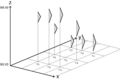
z

1

z

2

z

3

z

4

z

5

z

6

z

7

z

8

z

9

Figure 3: Node numbering convention in the neighbourhood of a central cellz9 (edited from: [39])

4.1. Methods of derivatives calculation

The basis of the derivatives determination is to calculate partial derivatives of the surface in two directions: North-South (denoted as^∂z_∂y with respect to the alignment with this axis) and East-West (denoted as ^∂z_∂x). There are several methods for calculation of those gradients, their comparison was performed in [23], [42] and also in [34]. The conclusion was that the 4-Cell method [15] provides the most precise results, closely followed by the Horn’s method [22]. The third best algorithm was a modified version of Horn’s method and as the forth the method of Sharpnack and Akin [33] was evaluated [23], these conclusions are approximately in agreement with the conclusions made in [34]. Study [42] was focused mainly on other elements of calculation. The algorithms were tested with respect to data quality and the resolution of the grid but findings from all these papers [23, 34, 42] suggest that

(29)

4-Cell, Horn’s, Sharpnack’s and Akin’s methods are all good estimators of the first derivatives of the surface. Based on these results, these three algorithms for gradient calculation are considered in the article, they happen to be the most commonly implemented in GIS.

In all upcoming formulas the cells are labelled according to Fig. 3. The variable d denotes the size of the grid cell. The arrangement and numbering of the cells vary through the literature and the formulas for calculation of the derivations vary accordingly [39].

The 4-Cell method calculates the values of gradients only from the cells that have direct neighbourhood with the central cell. The method was firstly described in [15]. The equations for this calculation are:

∂z

∂x = z2−z6

2d , (4.1a)

∂z

∂y = z8−z4

2d . (4.1b)

Horn’s method considers even the cells in the neighbourhood that have only one point common with the central cell. Cells that have common edge have been assigned higher weight in the calculation. The method was presented in [22] and the equations are:

∂z

∂x = (z1+ 2z2+z3)−(z7+ 2z6+z5)

8d , (4.2a)

∂z

∂y = (z7+ 2z8+z1)−(z5+ 2z4+z3)

8d . (4.2b)

Sharpnack and Akin’s Method is very similar to the Horn’s method with the change that all cells have the same weight. This method was proposed in [33] and the equations have the following form:

∂z

∂x =(z1+z2+z3)−(z7+z6+z5)

6d , (4.3a)

∂z

∂y =(z7+z8+z1)−(z5+z4+z3)

6d . (4.3b)

4.2. Calculation of slope and aspect

The three methods that were mentioned in the previous section provide three ways for the gradient calculation. These gradients are further used to calculate the slope S and the aspectA. For the slope calculation as a proportional rise the following equation is used:

S = s∂z

∂x 2

+ ∂z

∂y 2

. (4.4)

(30)

If the result should be in percent, a slightly different variation of the equation is needed:

S= 100 s∂z

∂x ²

+ ∂z

∂y ²

. (4.5)

If the result should be provided in degrees, a slight modification is necessary. This slope is labelled as geographical:

Sg (^◦) =180 π arctan



s

∂z

∂x 2

+ ∂z

∂y 2

. (4.6)

The calculation of aspect is a bit more complicated and requires the use of arctan2function:

A= arctan2(−∂z

∂y,−∂z

∂x). (4.7)

The mathematical aspectAis different from the geographical aspectAg,Ahas a range of [−π, π] radians, the value of 0 for the East and the values increase in a counter-clockwise direction. Ag has a range of [0,2π] in radians or [0^◦,360^◦] in degrees, the value of0for the North and the values increase in a clockwise direction [39]. So there is a need to adjust the values by this formula:

Ag (^◦) =

(450^◦−¹⁸⁰π A if ¹⁸⁰_π A >90^◦

90^◦−¹⁸⁰π A otherwise. (4.8)

Based on those equations the calculation of approximation of slope and aspect can be calculated from the surface represented by the grid.

5. First derivatives of fuzzy surfaces

In any analysis calculated on a fuzzy surface uncertainty of the surface is propagated through the analysis into the result. Such result then shows uncertainty connected to the input data represented as fuzzy numbers. So far there are three examples of the calculation of a fuzzy slope in the literature provided in [16], [37] and [6].

Unfortunately, in first two cases a fuzzy slope is not the main focus of the research so it is not discussed in detail. [16] use a fuzzy slope to identify the areas having a slope potentially higher than25 %, but the calculation serves as one of the several examples in the article, so it is discussed very briefly. [37] provided methods for the calculation of partial derivatives using the finite elements method, but the presented method is focused on a fuzzy surface constructed using purely triangular fuzzy numbers. The equations are adjusted to work on such surface, but it does not handle the calculation of a fuzzy slope in general, because triangular fuzzy numbers are only one type of a theoretically infinite set of fuzzy number types. These case

(31)

specific adjustments of equations are common for presenting methods that utilize fuzzy arithmetic [19]. [6] described the calculation of only fuzzy slope using Horn’s algortihm. There has been no attempt (of which the authors are aware) to calculate the aspect of a fuzzy surface.

The basis for the determination of both slope and aspect is the calculation of gradients ^∂z_∂x and ^∂z_∂y. Considering that all inputs are uncertain and represented by fuzzy numbers, the results will also contain uncertainty and they will also be represented by fuzzy numbers. The calculation of gradients themselves is based on basic arithmetic operators that have fuzzy equivalents according to Eqs. (2.2, 2.3) and ((2.5, 2.6). This applies for all three methods of the gradient calculation (Eqs.

(4.2, 4.1, 4.3)).

5.1. Slope

Calculating slope of a fuzzy surface according to Eqs. (4.5, 4.6) does not need any special approaches. Square of a fuzzy number can be calculated according to Eq.

(2.8) and square root is a monotonous function and can be calculated according to Eqs. (2.2) and (2.7). If the slope is to be provided in degrees then the Eq. (4.6) is used. As mentioned previously, there is no problem with using crisp numbers with fuzzy numbers while calculating. Thus obtaining the value of the slope as a fuzzy number is a relatively simple matter.

5.2. Aspect

The aspect calculation is more complicated then the slope calculation. The Eq.

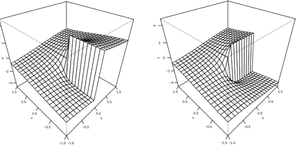
(4.7) contains the function arctan2 [18] that has to be calculated for two fuzzy arguments. This in not a trivial operation and the function has to be modified to allow the calculation. The common definition ofarctan2is:

arctan2(y, x) =











arctan^y_x ifx >0

arctan^y_x+π ify≥0andx <0 arctan^y_x−π ify <0andx <0 +^π₂ ify >0andx= 0

−^π2 ify <0andx= 0 undefined ify= 0andx= 0

(5.1)

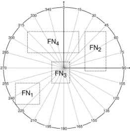
From the viewpoint of the calculation with fuzzy numbers there are two main problems. The function is not defined fory= 0andx= 0and it is discontinuous for x > 0 and y = 0 (Fig. 5). This complicates the calculation if Y˜ and X˜ contain 0. Figure 4 shows four examples of areas bounded by supports of fuzzy numbers, labelled FN1, FN2, FN3 and FN4. As visible from the examples, FN1

and FN2 delimit angle intervals with the values of approximately [215^◦,250^◦] and [30^◦,100^◦].¹ Example FN3 shows a situation in which both intervals contain 0

1The presented examples are for the sake of understanding shown in degrees with0^◦pointing