Contents
A. Bege, J. Bukor, J. T. Tóth, On (log-) convexity of power mean . . . 3 Cs. Biró, G. Kovásznai, A. Biere, G. Kusper, G. Geda, Cube-and-
Conquer approach for SAT solving on grids . . . 9 M. Grebenyuk, J. Mikeš, On normals of manifolds in multidimensional
projective space . . . 23 R. Király, Complexity metric based source code transformation of Erlang
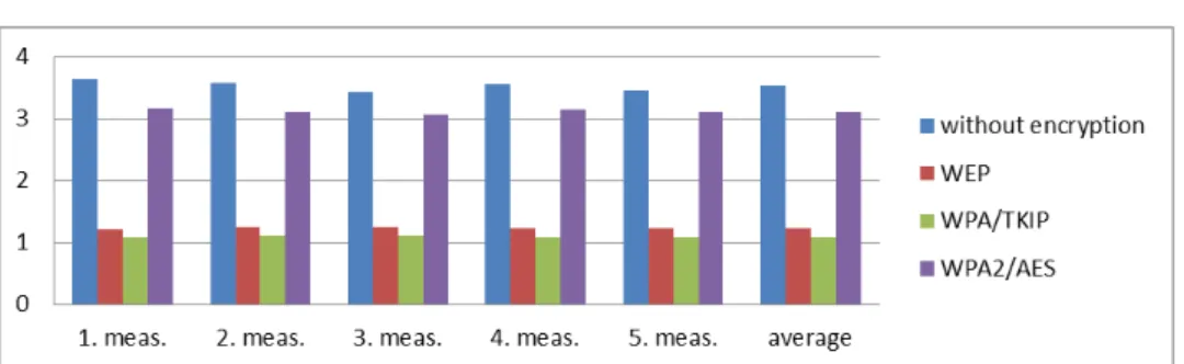
programs . . . 29 T. Krausz, J. Sztrik, Performance evaluation of wireless networks speed
depending on the encryption . . . 45 I. Kuzmina, J. Mikeš,On pseudoconformal models of fibrations determined
by the algebra of antiquaternions and projectivization of them . . . 57 F. Nagy, R. Kunkli, Method for computing angle constrained isoptic
curves for surfaces . . . 65 J. Pócsová,Note on formal contexts of generalized one-sided concept latti-
ces . . . 71 J. L. Ramírez,Bi-periodic incomplete Fibonacci sequences . . . 83 M. Shattuck,On the zeros of some polynomials with combinatorial coeffi-
cients . . . 93 Methodological papers
J. L. Cereceda, Averaging sums of powers of integers and Faulhaber poly- nomials . . . 105 M. I. Cîrnu,Linear recurrence relations with the coefficients in progression 119 E. Gyimesi, G. Nyul, A note on Golomb’s method and the continued
fraction method for Egyptian fractions . . . 129 T. Radványi, E. Kovács,Inserting RFID systems into the Software Infor-
mation Technology course . . . 135
ANNALESMATHEMATICAEETINFORMATICAE42.(2013)
TOMUS 42. (2013)
COMMISSIO REDACTORIUM
Sándor Bácsó (Debrecen), Sonja Gorjanc (Zagreb), Tibor Gyimóthy (Szeged), Miklós Hoffmann (Eger), József Holovács (Eger), László Kovács (Miskolc),
László Kozma (Budapest), Kálmán Liptai (Eger), Florian Luca (Mexico), Giuseppe Mastroianni (Potenza), Ferenc Mátyás (Eger),
Ákos Pintér (Debrecen), Miklós Rontó (Miskolc), László Szalay (Sopron), János Sztrik (Debrecen), Gary Walsh (Ottawa)
ANNALES MATHEMATICAE ET INFORMATICAE International journal for mathematics and computer science
Referred by
Zentralblatt für Mathematik and
Mathematical Reviews
The journal of the Institute of Mathematics and Informatics of Eszterházy Károly College is open for scientific publications in mathematics and computer science, where the field of number theory, group theory, constructive and computer aided geometry as well as theoretical and practical aspects of programming languages receive particular emphasis. Methodological papers are also welcome. Papers sub- mitted to the journal should be written in English. Only new and unpublished material can be accepted.
Authors are kindly asked to write the final form of their manuscript in LATEX. If you have any problems or questions, please write an e-mail to the managing editor Miklós Hoffmann: hofi@ektf.hu
The volumes are available athttp://ami.ektf.hu
MATHEMATICAE ET INFORMATICAE
VOLUME 42. (2013)
EDITORIAL BOARD
Sándor Bácsó (Debrecen), Sonja Gorjanc (Zagreb), Tibor Gyimóthy (Szeged), Miklós Hoffmann (Eger), József Holovács (Eger), László Kovács (Miskolc),
László Kozma (Budapest), Kálmán Liptai (Eger), Florian Luca (Mexico), Giuseppe Mastroianni (Potenza), Ferenc Mátyás (Eger),
Ákos Pintér (Debrecen), Miklós Rontó (Miskolc), László Szalay (Sopron), János Sztrik (Debrecen), Gary Walsh (Ottawa)
INSTITUTE OF MATHEMATICS AND INFORMATICS ESZTERHÁZY KÁROLY COLLEGE
HUNGARY, EGER
HU ISSN 1787-6117 (Online)
A kiadásért felelős az Eszterházy Károly Főiskola rektora Megjelent az EKF Líceum Kiadó gondozásában
Kiadóvezető: Czeglédi László Műszaki szerkesztő: Tómács Tibor Megjelent: 2013. december Példányszám: 30
Készítette az
Eszterházy Károly Főiskola nyomdája Felelős vezető: Kérészy László
On (log-) convexity of power mean
Antal Bege
a, József Bukor, János T. Tóth
b∗aDept. of Mathematics and Informatics, Sapientia Hungarian University of Transylvania,Targu Mures, Romania
bDept. of Mathematics and Informatics, J. Selye University, Komárno, Slovakia bukorj@selyeuni.sk,tothj@selyeuni.sk
Submitted October 20, 2012 — Accepted March 22, 2013
Abstract
The power meanMp(a, b) of orderp of two positive real valuesa andb is defined byMp(a, b) = ((ap+bp)/2)1/p, forp6= 0andMp(a, b) =√
ab, for p= 0. In this short note we prove that the power meanMp(a, b)is convex in pforp≤0, log-convex forp≤0and log-concave forp≥0.
Keywords:power mean, logarithmic mean MSC:26E60, 26D20
1. Introduction
Forp∈R, the power meanMp(a, b)of orderpof two positive real numbers,aand b, is defined by
Mp(a, b) =
( ap+bp 2
p1
, p6= 0
√ab, p= 0.
Within the past years, the power mean has been the subject of intensive research.
Many remarkable inequalities forMp(a, b)and other types of means can be found in the literature.
It is well known thatMp(a, b)is continuous and strictly increasing with respect top∈Rfor fixeda, b >0 witha6=b.
∗The second and the third author was supported by VEGA Grant no. 1/1022/12, Slovak Republic.
http://ami.ektf.hu
3
Note thatMp(a, b) =aMp(1,ab). Mildorf [3] studied the function f(p, a) =Mp(1, a) =
1 +ap 2
1p
and proved that for any given real numbera >0 the following assertions hold:
(A) for p≥1the function f(p, a)is concave inp, (B) forp≤ −1the functionf(p, a)is convex inp.
The aim of this note is to study the log-convexity of the power mean Mp(a, b)in variable p. As a consequence we get several known inequalities and their general- ization.
2. Main results
Theorem 2.1. Let f(p, a) =Mp(1, a). We have (i) forp≤0 the function f(p, a) is log-convex inp, (ii) forp≥0 the function f(p, a) is log-concave inp, (iii) forp≤0 the function f(p, a) is convex inp.
Proof. Observe that for any real numbertthere holds
f(pt, a)t=f(p, at). (2.1) Let
g(p, a) = lnf(p, a).
Taking the logarithm in (2.1) we have
tg(pt, a) =g(p, at).
Calculating partial derivatives of both sides of the above equation we get t2g01(pt, a) =g01(p, at)
and
t3g0011(pt, a) =g0011(p, at). (2.2) Specially, takingp= 1in (2.2), we have
t3g1100(t, a) =g0011(1, at). (2.3) Taking into account that the function f(p, a) is increasing and concave in p for p≥1 (see (A)), the functiong(p, a)is also increasing and concave inpforp≥1.
For this reason
g1100(1, at)≤0
for an arbitrary a >0 and realt. Let us consider the left hand side of (2.3). We have
t3g1100(t, a)≤0
which yields to the facts that the function g(p, a)is concave for p >0, therefore the function f(p, a) is log-concave in this case and the function g(p, a) is convex for p < 0. Hence the assertions (i), (ii) follow. Clearly, the assertion (iii) follows immediately from (i).
The following result is a consequence of the assertion (iii) Theorem 2.1.
Corollary 2.2. Inequality
αMp(a, b) + (1−α)Mq(a, b)≥Mαp+(1−α)q(a, b) (2.4) holds for all a, b >0,α∈[0,1]andp, q≤0.
Let us denote byG(a, b) = √
ab and H(a, b) = a+b2ab the arithmetic mean and harmonic mean of aand b, respectively. For α= 23, p= 0,q = 1 in (2.4) we get the inequality
2
3G(a, b) +1
3H(a, b)≥M−1
3(a, b) which was proved in [6].
The next result is a consequence of (ii) in Theorem 2.1.
Corollary 2.3. Forα∈[0,1],p, q≥0 the inequality
Mpα(a, b)Mq(1−α)(a, b)≤Mαp+(1−α)q(a, b) (2.5) holds for all a, b >0.
Let us denote byA(a, b) =a+b2 ,G(a, b) =√ ab,
L(a, b) = ( b
−a
lnb−lna, a6=b
a, a=b.
the arithmetic mean, geometric mean and logarithmic mean of two positive numbers aandb, respectively. Taking into account the result of Tung-Po Lin [2]
L(a, b)≤M1
3(a, b) (2.6)
together with (2.5) we have
Mpα(a, b)L(1−α)(a, b)≤Mαp+(1−α)1
3(a, b). (2.7)
Specially, forp= 1andp= 0in (2.7) we get the inequalities Aα(a, b)L(1−α)(a, b)≤M1+2α
3 (a, b)
and
Gα(a, b)L(1−α)(a, b)≤M1−α 3 (a, b) respectively, which results were published in [5].
Denote by
I(a, b) = (1
e aa bb
a−b1
, a6=b
a, a=b.
the identric mean of two positive integers. It was proved by Pittenger [4] that M2
3(a, b)≤I(a, b)≤Mln 2(a, b). (2.8) Using (2.5) together with (2.6) and (2.8) we immeditely have
Iα(a, b)L(1−α)(a, b)≤Mαln 2+(1−α)1
3.
Note, in the case ofα= 12 our result does not improve the inequality pI(a, b)L(a, b)≤M1
2(a, b)
which is due to Alzer [1], but our result is a more general one.
With the help of using Theorem 2.1 more similar inequalities can be proved.
3. Open problems
Finally, we propose the following open problem on the convexity of power mean.
The problem is to prove our conjecture, namely
a,b>0inf {p:Mp(a, b)is concave for variablep}= ln 2 2 , sup
a,b>0{p:Mp(a, b)is convex for variablep}= 1 2.
References
[1] Alzer, H., Ungleichungen für Mittelwerte,Arch. Math (Basel),47(5) (1986) 422–
426.
[2] Lin, T. P., The power mean and the logarithmic mean,Amer. Math. Monthly,81 (1974) 879–883.
[3] Mildorf, T. J., A sharp bound on the two variable power mean, Mathemat- ical Reflections, 2 (2006) 5 pages, Available online at [http://awesomemath.org/
wp-content/uploads/reflections/2006_2/2006_2_sharpbound.pdf]
[4] Pittenger, A. O., Inequalities between arithmetic and logarithmic means, Univ.
Beograd. Publ. Elektrotehn. Fak. Ser. Mat. Fiz.,678–715(1980) 15–18.
[5] Shi, M.-Y., Chu, Y.-M. and Jiang, Y.-P., Optimal inequalities among various means of two arguments,Abstr. Appl. Anal., (2009) Article ID 694394, 10 pages.
[6] Chu, Y.-M., Xia, W.-F.: Two sharp inequalities for power mean, geometric mean, and harmonic mean,J. Inequal. Appl.(2009) Article ID 741923, 6 pages.
Cube-and-Conquer approach for SAT solving on grids ∗
Csaba Biró
a, Gergely Kovásznai
b, Armin Biere
c, Gábor Kusper
a, Gábor Geda
aaEszterházy Károly College birocs,gkusper,gedag@aries.ektf.hu
bVienna University of Technology kova@forsyte.tuwien.ac.at
cJohannes Kepler University biere@jku.at
Submitted May 10, 2013 — Accepted December 9, 2013
Abstract
Our goal is to develop techniques for using distributed computing re- sources to efficiently solve instances of the propositional satisfiability problem (SAT). We claim that computational grids provide a distributed computing environment suitable for SAT solving. In this paper we apply the Cube and Conquer approach to SAT solving on grids and present our parallel SAT solver CCGrid(Cube and Conquer on Grid) on computational grid infrastructure.
Our solver consists of two major components. The master application runs march_cc, which applies a lookahead SAT solver, in order to partition the in- put SAT instance into work units distributed on the grid. The client applica- tion executes aniLingelinginstance, which is a multi-threaded CDCL SAT solver. We use BOINC middleware, which is part of the SZTAKI Desktop Grid package and supports the Distributed Computing Application Program- ming Interface (DC-API). Our preliminary results suggest that our approach can gain significant speedup and shows a potential for future investigation and development.
Keywords:grid, SAT, parallel SAT solving, lookahead, march_cc, iLingeling, SZTAKI Desktop Grid, BOINC, DC-API
∗Supported by Austro-Hungarian Action Foundation, project ID: 83öu17.
http://ami.ektf.hu
9
1. Introduction
Propositional satisfiability is the problem of determining, for a formula of the propo- sitional logic, if there is an assignment of truth values to its variables for which that formula evaluates to true. By SAT we mean the problem of propositional satisfiability for formulas in conjunctive normal form (CNF). SAT is one of the most-researched NP-complete problems [8] in several fields of computer science, including theoretical computer science, artificial intelligence, hardware design, and formal verification [5]. Also it should be noted that the hardness of the problem is caused by the possibly increasing number of the variables, since by a fixed set of variables SAT and n-SAT are regular languages and therefore there is a determin- istic (theoretical) linear time algorithm to solve them, see, [21, 23].
Modern sequential SAT solvers are based on the Davis-Putnam-Logemann- Loveland (DPLL) [9] algorithm. This algorithm performs Boolean constraint prop- agation (BCP) and backtrack search, i.e., at each node of the search tree it selects a decision variable, assigns a truth value to it, and steps back when conflict oc- curs. Conflict-driven clause learning (CDCL) [5, Chpt. 4] is based on the idea that conflicts can be exploited to reduce the search space. If the method finds a conflict, then it analyzes this situation, determines a sufficient condition for this conflict to occur, in form of a learned clause, which is then added to the formula, and thus avoids that the same conflict occurs again. This form of clause learning was first introduced in the SAT solverGRASP [19] in 1996. Besides clause learning, lazy data structures are one of the key techniques for the success of CDCL SAT solvers, such as “watched literals” as pioneered in 2001, by the CDCL solverChaff [20, 18] . Another important technique is the use of the VSIDS heuristics and the first-UIP backtracking scheme. In the state-of-the-art CDCL solvers, likePrecoSAT and Lingeling[3, 4], several other improvements are applied. Besides enhanced preprocessing techniques like e.g. failed literal detection, variable elimination, and blocked clause elimination, clause deletion strategies and restart policies have a great impact to the performance of the CDCL solver.
Lookahead SAT solvers [5, Chpt. 5] combine the DPLL algorithm with looka- heads, which are used in each search node to select a decision variable and at the same time to simplify the formula. One popular way of lookahead measures the effect of assigning a certain variable to a certain truth value: BCP is applied, and then the difference between the original clause set and the reduced clause set is measured (by using heuristics). In general, the variable for which the lookahead onboth truth values results in a large reduction of the clause set is chosen as the decision variable. The first lookahead SAT solver was posit [10] in 1995. It al- ready applied important heuristics for pre-selecting the “important” variables, for selecting a decision variable, and for selecting a truth value for it. The lookahead solverssatz [17] andOKsolver [16] further optimized and simplified the heuristics, e.g.,satz does not use heuristics for selecting a truth value (rather preferstrue), andOKsolverdoes not apply any pre-selection heuristics. Furthermore,OKsolver added improvements like local learning and autarky reasoning. In 2002, the solver
march [13] further improved the data structures and introduced preprocessing tech- niques. As a variant of march,march_cc[14] can be considered as a case splitting tool. It produces a set of cubes, where each cube represents a branch cutoff in the DPLL tree constructed by the lookahead solver. It is also worth to mention that march_cc outputs learnt clauses as well, which represent refuted branches in the DPLL tree. The resulting set of cubes represents the remaining part of the search tree, which was not refuted by the lookahead solver itself.
There are two types of basic appearance of parallelism in computations, the
“and-parallelism” and the “or-parallelism” [22]. The first is used in high perfor- mance computing, while the latter is more similar to nondeterministic guesses (data parallel). SAT can (theoretically effectively) be solved by several new com- puting paradigms using or-parallelism and by using, roughly speaking, exponential number of threads. Since multi-core architectures are common today, the need for parallel SAT solvers using multiple cores has increased considerably.
In essence, there are two approaches to parallel SAT solving [12]. The first group of solvers typically follow a divide-and-conquer approach. They split the search space into several subproblems, sequential DPLL workers solve the subproblems, and then these solutions are combined in order to create a solution to the original problem. This first group uses relatively intensive communication between the nodes. They do for example load balancing, and dynamic sharing of learned clauses.
The second group apply portfolio-based SAT solving. The idea is to run inde- pendent sequential SAT solvers with different restart policies, branching heuristics, learning heuristics, etc. ManySAT [11] was the first portfolio-based parallel SAT solver. ManySAT applies several strategies to the sequential SAT solver MiniSAT.
Plingeling[3, 4] follows a similar approach, and uses the sequential SAT solver Lingeling. In most of the state-of-the-art portfolio-based parallel SAT solvers (e.g. ppfolio, pfolioUZK, SATzilla) not only different strategies, but even dif- ferent sequential solvers compete and, to a limited extent, cooperate on the same formula. In such approaches there is no load balancing and the communication is limited to the sharing of learned clauses.
GridSAT[7, 6] was the first complete and parallel SAT solver employing a grid.
It belongs to the divide-and-conquer group. It is based on the sequential SAT solver zChaff. Besides achieving significant speedup in the case of some (satisfiable and even unsatisfiable) instances, GridSAT is able to solve some problems for which sequential zChaff exceeds time out. GridSAT distributes only the short learned clauses over the nodes, therefore it minimizes the communication overhead. Search space splitting is based on the selection of a so-called pivot variable x on the second decision level, and then creating two subproblems by adding a new decision on x resp. ¬xto the first decision level. If sufficient resources are available, the subproblems can further be partitioned recursively. Each new subproblem is defined by a clause set, including learned clauses, and a decision stack.
[15] proposes a more sophisticated approach, based on using “partition func- tions”, in order to split a problem into a fixed number of subproblems. Two par- tition functions were compared, a scattering-based and a DPLL-based one with
lookahead. A partition function can be applied even in a recursive way, by repar- titioning difficult subproblems (e.g., the ones that exceeds time out). For some of the experiments, an open source grid infrastructure called Nordugrid was used.
SAT@home[25] is a large volunteer SAT-solving project on grid, which involves more than 2000 clients. The project is based on the Berkeley Open Infrastruc- ture for Network Computing (BOINC) [1], which is an open source middleware system for volunteer grid computing. On top of BOINC, the project was imple- mented by using the SZTAKI Desktop Grid [24], which provides the Distributed Computing Application Programming Interface (DC-API), in order to simplify the development, and then also to deploy and distribute applications to multiple grid environments. [25] proposes a rather simple partitioning approach: given a set of nselected variables, called a decomposition, a set of2n subproblems is generated.
The key issue is how to select a decomposition. One way to solve this issue, is to derive the set of “important” decomposition variables from the original problem formulation, which, however, then is problem-specific, and needs human guidance.
For instance, in the context of SAT-based cryptoanalysis of keystream generators, a decomposition set can be obtained from the encoding of the initial state of the linear feedback shift registers [25]. SAT@homeuses no data exchange among clients.
Our approach, calledCCGrid, also uses BOINC and the SZTAKI Desktop Grid, as it is detailed in Sect. 3, but is based on the Cube and Conquer approach [14].
For partitioning the input problem, we usemarch_cc. Our approach differs from the previous ones in the fact that it uses a parallel SAT solver, iLingeling, for solving the particular subproblems, on each client. In Sect. 4 we present some experiments and preliminary results.
2. Preliminaries
Given a Boolean variable x, there exist twoliterals, the positive literalxand the negative literal x. A clause is a disjunction of literals, acube is a conjunction of literals. Either a clause or a cube can be considered as a finite set of literals.
Atruth assignment for a (finite) clause set or cube set F is a function φthat maps literals in F to {0,1}, such that if φ(x) = v, then φ(x) = 1−v. A clause resp. cubeC is satisfied by φifφ(l) = 1for some resp. everyl ∈C. A clause set resp. cube setF is satisfied by φifφsatisfiesC for every resp. someC∈F.
For representing the input clause set for a SAT solver, the DIMACS CNF format is commonly used, which references a Boolean variable by its (1-based) index. A negative literal is referenced by the negated reference to its variable. A clause is represented by a sequence of the references to its literals, terminated by a “0”.
The iCNF format extends the CNF format with a cube set.1 A cube, called an assumption, is represented by a leading character “a” followed by the references to its literals and a terminating “0”.
1http://users.ics.tkk.fi/swiering/icnf/
3. Architecture
Our application is a variant of the Cube and Conquer approach [14] and consists of two major components: a master application and a client application. The master is responsible for dividing the global input data into smaller chunks and distributing these chunks in the form of work units. Interpreting the output generated by the clients out of the work units and combining them to form a global output is also the job of the master. The architecture is depicted in Fig. 1. Similar to [25], the environment for running our system is the SZTAKI Desktop Grid [24] and BOINC [1], and was implemented by the use of the DC-API.
database BOINC
Server march_cc
BOINC deamons work units
BOINC Client iLingeling
PC1
BOINC Client iLingeling
PC2
. . .
BOINC Client iLingeling
PCn
Figure 1: CCGrid architecture
The master
The master executes a partitioning tool called march_cc [14], which is based on the lookahead SAT solver march. Given a CNF file, march_cc primarily tries to refute the input clause set. If this does not succeed, march_cc outputs a set of assumptions (cubes) that describe the cutoff branches in the DPLL tree. These assumptions cover all subproblems of the input clause set that have not been refuted during the partitioning procedure. Given these assumptions, the master application creates work units, each of which consists of the input CNF file and a slice of the
assumption set. As it can be seen in Fig. 2, if one of the clients reports one of the work units to be satisfiable, then the master outputs the satisfying model and destroys all the running work units. If every clients report unsatisfiability, then the master outputs unsatisfiability.
SAT Running
. . .
Running UNSAT UNSAT
. . .
UNSAT Figure 2: (a) If the problem is SAT, it is enough to find a SAT
derived instance. (b) If the problem is UNSAT, one must show all derived instances UNSAT.
The pseudocode below shows how the master application works. It is divided into three procedures; the Main procedure is shown in Algorithm 1. It shares two constants with the other procedures: (i)maxAsmCount defines the maximum number of assumptions per work unit; (ii) rfsInterval gives a refresh interval at which DC-API events are processed. The master application uses several global variables; all of them are self-explanatory. In loop 6-9, work units are created, by calling the procedureCreateWorkUnit. Loop 10-13 then processes DC-API events generated by those work units that have finished solving their subproblems.
Processing DC-API events is done by calling a callback function which has been previously set to ProcessWorkUnitResult in line 3. The loop stops if either one of the work units returns a SAT result or all the work units completed.
CreateWorkUnit, shown in Algorithm 2, creates and submits a work unit to the grid. First, the CNF file is added to the new work unit. Then, in the loop, at most maxAsmCount assumptions from asmFile are copied into the new file asmChunkFile. Note thatasmFile is global, it has been opened by the Main procedure (Algorithm 1, line 4), and therefore its current file position is held.
Finally, asmChunkFile is added to the work unit, which is then submitted to the grid.
As already mentioned, ProcessWorkUnitResult, shown in Algorithm 3, works as a callback function for DC-API events. It processes the result returned by a work unit.
Algorithm 1 Master: main procedure
Require: global constantsmaxAsmCount,rfsInterval
Require: global variablescnfFile,asmFile,wuCount,res,resFile 1: procedureMain
2: initialize DC-API master
3: setProcessWorkUnitResultas result callback 4: openasmFile
5: wuCount←0
6: while notEOF(asmFile)do 7: CreateWorkUnit 8: wuCount←wuCount+ 1 9: end while
10: whileres6=SATandwuCount>0do 11: waitrfsInterval
12: process DC-API events 13: end while
14: if res6=SATthen
15: res←UNSAT
16: cancel all work units 17: end if
18: end procedure
Algorithm 2 Master: creating work units
1: procedureCreateWorkUnit 2: wu←new work unit 3: wu.cnfFile←cnfFile 4: asmChunkFile←new file 5: for i←1tomaxAsmCountdo 6: if EOF(asmFile)then
7: break
8: end if
9: copy next assumption fromasmFiletoasmChunkFile 10: i←i+ 1
11: end for
12: wu.asmFile←asmChunkFile 13: submitwuto the grid 14: end procedure
Algorithm 3 Master: processing work unit result
1: procedureProcessWorkUnitResult(wu) 2: if wu.res=SATthen
3: res←SAT
4: copywu.resFiletoresFile 5: end if
6: wuCount←wuCount−1 7: end procedure
The client
Each client executes the parallel CDCL solveriLingeling[14, 4], for a fixed num- ber of threads. Each thread executes a separatelingelinginstance. iLingeling expects as input an iCNF file, including 1 or more assumptions, which is then loaded into a working queue. Eachlingelinginstance reads the input clause set, and then, in each iteration, gets the first assumption from the working queue.
If one of the lingeling instances can prove that the clause set is satisfiable under the given assumptions, theniLingelingreports that the clause set itself is satisfiable, the satisfying model is returned, and hence the remaining assumptions in the working queue can be ignored. Otherwise, i.e., if a lingeling instance reports unsatisfiability, then the assumption is retrieved from the working queue and the same SAT solver instance continues with the solving procedure. If the working queue becomes empty, theniLingelingreports that the clause set under the given set of assumptions is unsatisfiable.
Algorithm 4 shows the client’s main procedure. It uses one global constant, thrCount, which specifies the number of worker threads to use. First, the procedure creates aniLingelinginstance withthrCountworker threads, loads both the CNF and the assumption files, and runs iLingeling. In loop 7-12, the results by all the threads are checked: if any of them is SAT then the result for the work unit is SAT; otherwise it is UNSAT (line 14). The result, as well as the satisfying model, is written into a result file by the procedure CreateResultFile, shown in Algorithm 5.
Algorithm 4 Client: main procedure Require: global constantthrCount
1: procedureMain(wu) 2: initialize DC-API client
3: iLingeling ←new iLingeling instance usingthrCount threads 4: loadwu.cnfFileintoiLingeling
5: loadwu.asmFileintoiLingeling 6: runiLingeling
7: for i←1tothrCountdo
8: if ith thread’s result is SATthen
9: wu.res←SAT
10: break
11: end if 12: end for
13: if i >thrCountthen 14: wu.res←UNSAT 15: end if
16: CreateResultFile(wu,iLingeling) 17: end procedure
Algorithm 5 Client: creating result file
1: procedureCreateResultFile(wu,iLingeling) 2: resFile←new file
3: writewu.resintoresFile 4: if wu.res=SATthen
5: model←satisfying assignment fromiLingeling 6: writemodelintowu.resFile
7: end if
8: wu.resFile←resFile 9: end procedure
4. Results and testing environment
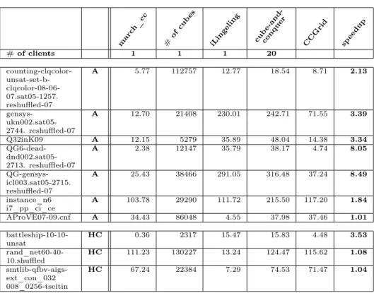
Our implementation consists of a quad-core SUN server with 6 GB memory, used as a master, and 20 quad-core PCs with 2 GB memory, used as clients. In our experiments, we used instances from the SAT Challenge 2012, from the Application (SAT + UNSAT) and the Hard Combinatorial (SAT + UNSAT) tracks. Results are presented in Tab. 1 and Tab. 2. The 1st column represents the instance’s name.
In the 2nd column, A resp. HC denotes Application resp. Hard Combinatorial problems. The 4th column shows the number of cubes, generated by march_cc.
The 3rd resp. 5th column shows the runtime of march_ccresp.iLingeling, being executed on the master. The 6th column contains the sum of the previous two numbers, which represents the overall runtime of the cube-and-conquer approach running on a single (quad-core) machine. The total runtime of CCGrid is shown in the 7th column, while the 8th column measures the speedup as the ratio of the runtimes in the 6th and 7th columns.
In our approach,CCgridhave been executed without any communication among clients. Even though they do not cooperate and do not exchange learnt clauses, CCGrid shows a wide range of speedups. We achieved speedup up to ca. 8.5 on UNSAT instances (QG-gensys-icl003.sat05-2715.reshuffled-07) and up to ca. 7 on SAT instances (sgen1-sat-160-100).
Since the master has to distribute quite large work units over the network, com- munication overhead matters in the case of small instances, where communication costs are significant compared to the input size. Therefore, although we used a 1Gbps LAN in our experiments, cube-and-conquer running on a single machine outperformedCCgridon some instances. If we look at thebattleship-16-31-sat row in Tab. 1, we can see that march_ccandiLingelingcan solve this problem on 1 client a bit faster thanCCGrid on 20 clients.
In the case of satisfiable instances, we might be lucky, finding a model quickly, or unlucky. If there are many satisfying models, then it is not worth to distribute the problem over many clients. However, if there exist only a few models, then it is a good idea to use many clients, since the more clients we use, the more probable it is for a client to be lucky enough to find one of those few solutions. Unfortunately, we have no information about how many models the instances in Tab. 1 have.
marc h_cc
#ofcub es
iLingeling cub e-and-
conquer CCGrid speedup
# of clients 1 1 1 20
vmpc_26 A 8.38 296 40.22 48.6 13.64 3.56
AProVE09-07 A 65.93 4245 19.12 85.05 79.16 1.07
clauses-4 A 29.68 25 59.01 88.69 81.98 1.08
gss-16-s100 A 155.28 6292 201.21 356.49 171.71 2.08
IBM_FV_
2004_rule_
batch_22 _SAT_dat. k65
A 17.93 361 148.95 166.88 154.02 1.08
ezfact64_3. sat05-
450. reshuffled-07 HC 458.71 469428 63.71 522.42 505.72 1.03
sgen1-sat-160-100 HC 10.65 210168 419.92 430.57 62.28 6.91
em_7_4 _8_exp HC 20.06 19419 170.9 190.96 46.47 4.11
battleship-16-31-
sat HC 174.89 91757 2.69 177.58 180.89 0.98
Hidoku_ enu_6 HC 125.02 256225 91.61 216.63 159.31 1.36
Table 1: Runtimes and speedup all instances are SAT
CCGridseems to be much better in distributing satisfiable instances from the HCtrack than the ones from theAtrack, sincemarch_ccseems to generate much more cubes for the previous ones.
In the case of unsatisfiable instances, we cannot be lucky to find an early solution since there is no satisfying model. When comparing the speedups in Tab. 1 and Tab. 2, we can see that speedups around 1 are more frequent on satisfiable instances.
This shows that in the case of unsatisfiable instances there is less risk of wasting resources without any speedup.
5. Future work and conclusion
This paper presents a first attempt of applying the Cube and Conquer approach [14]
to computational grids. We presented the parallel SAT solverCCGrid, which runs on the MTA SZTAKI Grid using BOINC. In this version, the master application appliesmarch_cc, using a lookhead solver, to split a SAT instance. The client ap- plication uses the parallel SAT solveriLingelingto deal with several assumptions.
The client creates a separateiLingelinginstance for each work unit, and destroys it after completing the work unit. For the sake of improving our current results, in future work, we would like to preserve the state of iLingelinginstances, including learnt clauses.
In our experience, the cube generation phase implemented inmarch_ccmakes up a significant part of the runtime. As a consequence, we were mostly able to achieve significant speedup on such instances on which the cube generation phase
marc h_cc
#ofcub es
iLingeling cub e-and-
conquer CCGrid speedup
# of clients 1 1 1 20
counting-clqcolor- unsat-set-b- clqcolor-08-06- 07.sat05-1257.
reshuffled-07
A 5.77 112757 12.77 18.54 8.71 2.13
gensys- ukn002.sat05- 2744. reshuffled-07
A 12.70 21408 230.01 242.71 71.55 3.39
Q32inK09 A 12.15 5279 35.89 48.04 14.38 3.34
QG6-dead- dnd002.sat05- 2713. reshuffled-07
A 2.38 12147 35.79 38.17 4.74 8.05
QG-gensys- icl003.sat05-2715.
reshuffled-07
A 25.43 38466 291.05 316.48 37.24 8.49
instance_n6
i7_pp_ci_ce A 103.78 29290 111.72 215.50 117.20 1.84
AProVE07-09.cnf A 34.43 86048 4.55 37.98 37.46 1.01
battleship-10-10-
unsat HC 0.36 2317 15.47 15.83 4.48 3.53
rand_net60-40-
10.shuffled HC 111.23 130227 13.24 124.47 115.62 1.08
smtlib-qfbv-aigs- ext_con_032 008_0256-tseitin
HC 67.24 22384 7.29 74.53 71.47 1.04
Table 2: Runtimes and speedup all instances are UNSAT
took a relatively short time. Therefore, our further aim to reduce the time spent on cube generation by parallelizing the look-ahead solver. We plan to adaptmarch_cc to a cluster infrastructure and to investigate the possibility of merging our BOINC- based approach with a cluster-based master application. We expect further im- provement by analyzing the generated cubes and then, based on the result of the analysis, partitioning the cube set in a more sophisticated way.
In order to achieve larger speedup on unsatisfiable instances, it might be useful to call march_cc not only while partitioning the original problem, but also for repartitioning difficult subproblems, e.g., those on which a client exceeds a certain time limit. Finally, it might be interesting to apply similar techniques not only to clusters resp. grids, but also to cloud computing platforms.
References
[1] D. P. Anderson, BOINC: A System for Public-Resource Computing and Storage.
Proc. of GRID 2004, pp. 4–10, 2004.
[2] A. Balint, A. Belov, D. Diepold, A. Gerber, M. Järvisalo, C. Sinz (eds), Proceedings of SAT Challenge 2012: Solver and Benchmark Descriptions. Depart- ment of Computer Science Series of Publications B, vol. B-2012-2, University of Helsinki, 2012.
[3] A. Biere, Lingeling, Plingeling, PicoSAT and PrecoSAT at SAT Race 2010. Tech- nical Report 10/1, FMV Reports Series, JKU, 2010.
[4] A. Biere, Lingeling and Friends Entering the SAT Challenge 2012.Haifa Verification Conference,Department of Computer Science Series of Publications B, vol. B-2012-2, pp. 33–34, 2012.
[5] A. Biere, M. Heule, H. van Maaren, T. Walsh, Handbook of Satisfiability.
IOS Press, Amsterdam, 2009.
[6] W. Chrabakh, R. Wolski, GridSAT: A Chaff-based Distributed SAT Solver for the Grid.Proc. of SC’03, pp. 37–49, 2003.
[7] W. Chrabakh, R. Wolski, GrADSAT: A Parallel SAT Solver for the Grid. Tech- nical report, UCSB Computer Science, 2003.
[8] S. A. Cook, The Complexity of Theorem-Proving Procedures. Proc. of STOC’71, pp. 151–158, 1971.
[9] M. Davis, G. Logemann, D. Loveland, A Machine Program for Theorem Prov- ing.Commun. ACM, vol. 5, no. 7, pp. 394–397, 1962.
[10] J.W. Freeman, Improvements to Propositional Satisfiability Search Algorithms.
Ph.D. Dissertation, Department of Computer and Information Science, University of Pennsylvania, May, 1995.
[11] Y. Hamadi S. Jabbour, L. Sais, ManySAT: a Parallel SAT Solver. Journal on Satisfiability, Boolean Modeling and Computation, vol. 6, pp. 245–262, 2009.
[12] Y. Hamadi, S. Jabbour, C. Piette, L. Saïs, Deterministic Parallel DPLL.JSAT, vol. 7. no. 4, pp. 127–132, 2011.
[13] M. Heule, March: Towards a Look-ahead SAT Solver for General Purposes. Master thesis, TU Delft, The Netherlands, 2004.
[14] M. Heule, O. Kullmann, S. Wieringa, A. Biere, Cube and Conquer: Guiding CDCL SAT Solvers by Lookaheads.Proc. of Haifa Verification Conference,Lecture Notes in Computer Science, vol. 7261, pp. 50–65, 2011.
[15] A. E. J. Hyvärinen, T. Junttila, I. Niemelä, Partitioning SAT instances for distributed solving.Proc. of LPAR’10, pp. 372–386, 2010.
[16] O. Kullmann, Investigating the Behaviour of a SAT Solver on Random Formulas.
Technical Report CSR 23-2002, Swansea University, Computer Science Report Series, October, 2002.
[17] C.M. Li and Anbulagan, Look-Ahead versus Look-Back for Satisfiability Prob- lems.Lecture Notes in Computer Science, vol. 1330, pp. 342–356, 1997.
[18] Y. S. Mahajan, Z. Fu, S. Malik, Zchaff2004: An Efficient SAT Solver.Lecture Notes in Computer Science: Theory and Applications of Satisfiability Testing, vol.
3542, pp. 360–375, 2005.
[19] J. P. Marques-Silva, K. A. Sakallah, GRASP: A New Search Algorithm for Satisfiability.Proc. of ICCAD’96, pp. 220–227, 1996.
[20] M. W. Moskewicz, C. F. Madigan, Y. Zhao, L. Zhang, S. Malik, Chaff:
Engineering an Efficient SAT Solver.Proc. of DAC’01, pp. 530–535, 2001.
[21] B. Nagy, The Languages of SAT and n-SAT over Finitely Many Variables are Reg- ular.Bulletin of the EATCS, no. 82, pp. 286–297, 2004.
[22] B. Nagy, On the Notion of Parallelism in Artificial and Computational Intelligence.
Proc. of HUCI 2006, pp. 533–541, 2006.
[23] B. Nagy, On Efficient Algorithms for SAT.Proc. of CMC 2012, Lecture Notes in Computer Science, vol. 7762, pp. 295–310, 2013.
[24] P. Kacsuk, J. Kovács, Z. Farkas, A. C. Marosi, G. Gombás, Z. Balaton, SZTAKI Desktop Grid (SZDG): A Flexible and Scalable Desktop Grid System.Jour- nal of Grid Computing, vol. 7, no. 4, pp. 439–461, 2009.
[25] M. Posypkin, A. Semenov, O. Zaikin, Using BOINC Desktop Grid to Solve Large Scale SAT Problems.Computer Science, vol. 13, no. 1, pp. 25–34, 2012.
On normals of manifolds in multidimensional projective space ∗
Marina Grebenyuk
a, Josef Mikeš
baNational Aviation University, Kiev, Ukraine ahha@i.com.ua
bPalacky University Olomouc, Czech Republic josef.mikes@upol.cz
Submitted December 4, 2012 — Accepted January 31, 2013
Abstract
In the paper the regular hyper-zones in the multi-dimensional non-Eucli- dean space are discussed. The determined bijection between the normals of the first and second kind for the hyper-zone makes it possible to construct the bundle of normals of second-kind for the hyper-zone with assistance of certain bundle of normals of first-kind and vice versa. And hence the bundle of the normals of second-kind is constructed in the third-order differential neighbourhood of the forming element for hyper-zone. Research of hyper- zones and zones in multi-dimensional spaces takes up an important place in intensively developing geometry of manifolds in view of its applications to mechanics, theoretical physics, calculus of variations, methods of optimiza- tion.
Keywords: non-Euclidean space, regular hyper-zone, bundle of normals, bi- jection
MSC:53B05
1. Introduction
In this article we analyze the theory of regular hyper-zone in the extended non- Euclidean space. We derive differential equations that define the hyper-zone SHr
∗Supported by grant P201/11/0356 of The Czech Science Foundation.
http://ami.ektf.hu
23
with regards to a self-polar normalised frame of space λSn. The tensors which determine the equipping planes in the third-order neighborhood of the hyper-zone are introduced. The bundles of the normals of the first and second kind are con- structed by an inner invariant method in the third-order differential neighbourhood of the forming element for hyper-zone. The bijection between the normals of the first and second kind for the hyper-zoneSHr is determined.
The concept of zone was introduced by W. Blaschke [1]. V. Wagner [7] was the first who proposed to consider the surface equipped with the field of tangent hyper-planes in then-dimensional centro-affine space.
We apply the group-theoretical method for research in differential geometry developed by professor G.F. Laptev [4]. At present the method of Laptev remains the most efficient way of research for manifolds, immersed in generalized spaces.
We use results obtained in the article [3].
For the past years the methods of generalizations of Theory of regular and sin- gular hyper-zones (zones) with assistance of the Theory of distributions in multidi- mensional affine, projective spaces and in spaces with projective connections were studied by A.V. Stolyarov, Y.I. Popov and M.M. Pohila. In this article we analyze the theory of regular hyper-zone in the extended non-Euclidean space. We derive differential equations that define the hyper-zone SHr with regards to a self-polar normalised frame of spaceλSn. The tensors which determine the equipping planes in the third-order neighborhood of the hyper-zone are introduced. The bundles of the normals of the first and second kind are constructed by an inner invariant method in the third-order differential neighbourhood of the forming element for hyper-zone. The bijection between the normals of the first and second kind for the hyper-zoneSHris determined.
Before M. Grebenyuk and J. Mikeš in the article [2] discussed the theory of the linear distribution in affine space. The bundles of the projective normals of the first kind for the equipping distributions are constructed by an inner invariant method in second and third differential neighbourhoods of the forming element.
In the article we apply the group-theoretical method for research in differential geometry developed by G.F. Laptev [4]. At present the method of Laptev remains the most efficient way of research for manifolds, immersed in generalized spaces.
We use results obtained in the article [3].
2. Definition of the hyper-zone in the extended non- Euclidean space
Let a non-degenerated hyper-quadric be given in a projectiven-dimensional space Pn as
qIJ0 xIxJ= 0, q0IJ=q0JI, detkqIJ0 k 6= 0, I, J = 0,1, . . . , n,
where the smallest number of the coefficients of the same sign is equal toλ. Thus, it is possible to determine a subgroup of collineations for spacePn, which are preserv- ing this hyper-quadric and, hence, it is possible to introduce a projective metrics.
Let us name the obtained in this way metric space with this fundamental group as the extended non-Euclidian spaceλSn with indexλ[5], and the corresponding hyper-quadric as the absolute of the spaceλSn.
Let us consider a plane element(A, τ)in the spaceλSn which is composed of a pointAand a hyper-plane τ, where point Abelongs to planeτ.
Definition 2.1. Suppose that the point A defines an r-dimensional surface Vr
and the hyper-planeτ(A)is tangent to the surfaceVrin the corresponding points A ∈ Vr. Then the r-parametric manifold of the plane elements (A, τ) is called r-parametric hyper-zone SHr ⊂ λSn. The surface Vr is called the base surface and the hyper-planes τ(A) are called the principal tangent hyper-planes to the hyper-zoneSHr.
Definition 2.2. The characteristic planeXn−r−1(A)for the tangent hyper-plane τ =τ(u1, . . . , ur)is called thecharacteristic plane for the hyper-zonesSHr at the pointA(u1, . . . , ur).
Definition 2.3. The hyper-zoneSHr is called regular if the characteristic plane Xn−r−1(A) and the tangent plane Tr(A) for directing surface Vr for hyper-zone SHrat each pointA∈Vrhave no common straight lines.
The regular hyper-zoneSHr in a self-polar normalized basis {A0, A1, . . . , An} in the spaceλSn is defined as follows:
ωon= 0, ωoα= 0, ωnα= 0, ωon= 0, ωnα= 0, ωoα= 0, ωin=aijωj, ωαi =biαjωj, ωiα=bαijωj, ωio=−εoiωi, ωin=εinaijωj,
∇aij=−aijωnn−aijkωk, ∇biαj =biαjkωk, ∇bαij =bαijkωk, where
biαjai` =biα`aij, bαik=−εαibijaajk, biαk=bijαajk, and functionsbiαjk are symmetric according to indicesj and k.
Systems of objects
Γ2={aij, biαj}, Γ3={Γ2, aijk, biαjk}
make up fundamental objects of second and third orders respectively for hyper-zone SHr⊂λSn.
3. Canonical bundle of projective normals for the hyper-zone
With the help of the components of fundamental geometric object of the third order for hyper-zoneSHr⊂λSn let us construct the quantities
di= 1
r+ 2 aijkajk, ∇δdi = 0, di= 1
r+ 2 aijkajk, ∇δdi =diπnn.
The tensorsdianddi define dual equipping planes in the third-order neighborhood of the hyper-zoneSHr
Er−1≡[Mi] = [Ai+diAo], En−r≡[σi] = [τi+diτn].
Using the Darboux tensor
Lijk=aijk−a(ijdk), one builds the symmetric tensor
Lij =ak`ampLikmLj`p, ∇δLij= 0, which is non-degenerate in general case.
Let us consider a field of straight lines associated with the hyper-zoneSHr
h(Ao) = [Ao, P], P =An+xiAi+xαAα,
where each line passes through the respective pointA of the directing surface Vr
and do not belong to the tangent hyper-planeτ(Ao).
Let us require that straight lineh= [Ao, P]is an invariant line, i.e. δh=θh. The last condition is equivalent to the differential equations:
∇δχα=χαπnn and ∇δχi=χiπnn.
First equations are realized on the condition thatxα=Bα, and second equations have two solutions:
xi=−di, xi=Bi.
Hence, the system of the differential equations has a general solution of the following form:
xi =−di+σ(Bi+di), whereσ is the absolute invariant.
Thus, we obtain the bundle of straight lines, which is associated with the hyper- zoneSHrby inner invariant method:
h(σ) = [Ao, P(σ)] = [Ao, An+{(σ−1)di+σBi}Ai+BαAα], whereσ is the absolute invariant.
The constructed projective invariant bundle of straight lines makes it possible to construct the invariant bundle of first-kind normals En−r, which is associated by the inner method with the hyper-zoneSHr in the differential neighborhood of the third order of its generatrix element.
Consequently, it is possible to represent each invariant first kind normalEn−r(Ao) as the(n−r)-plane that encloses the invariant straight lineh(Ao)and the charac- teristicXn−r−1(Ao)for hyper-zoneSHr [6].
En−r(σ)def= [Xn−r−1(Ao); An+{(σ−1)di+σBi}Ai+BαAα, whereσ is the absolute invariant.
4. Bijection between first- and second-kind normals of the hyper-zone SH
rLet us introduce the correspondence between the normals of the first- and second- kind for the hyper-zone SHr. For that, let us construct a tensor:
Pi=−aijνj+di, ∇δPj= 0 (4.1) whereνj is the tensor satisfying the condition∇δνj =νjπnn.
The tensor Pi defines the normal of second-kind for hyper-zone SHr that is determined by the points
Mi=Ai+χiAo, ∇δχi= 0.
Further, the tensorνj can be represented using the components of the tensor Pi as follows
νj=−Piaij+dj.
Therefore, the bijection between the normals of the first- and second-kind for the hyper-zoneSHris obtained using the relations (4.1). The constructed bijection makes it possible to determine the bundle of second-kind normals, using the bundle of first-kind normals and vice versa. Therefore, we got constructed the bundle of second-kind normals, which is associated by the inner method with the hyper-zone SHr in the differential neighborhood of the third order of its generating element.
So true the following theorem.
Theorem 4.1. Tensor Pi defines the bijection between the normals of the first- and second-kind for the hyper-zone SHr.
Finally, we get the theorem.
Theorem 4.2. Tensorνj=−Piaij+didefines the bundle of second- kind normals, which is associated by inner method with the hyper-zone SHr in the differential neighborhood of the third order of its generating element.
References
[1] Blaschke, W.,Differential geometry, I. OSTI, M., L., (1935).
[2] Grebenyuk, M., Mikeš, J., Equipping Distributions for Linear Distribution,Acta Palacky Univ. Olomuc., Mathematica, 46 (2007) 35–42.
[3] Kosarenko, M. F., Fields of the geometrical objects for regular hyper-zoneSHr⊂
λSn, (Russian), Differential geometry of manifolds of figures.Interuniversity subject collection of scientific works. Kaliningrad Univ., 13 (1982) 38–44.
[4] Laptev, G. F., Differential geometry of embedded manifolds: group-theoretical method for research in differential geometry,Proc. of the Moscow Math. Soc., 2 (1953) 275–382.
[5] Rozenfeld, B. A., Non-Euclidean geometries,Gostechizdat, Moscow, (1955).
[6] Stoljarov, A. V., Differential geometry of zones, Itogi Nauki Tekh., Ser. Probl.
Geom., 10 (1978) 25–54.
[7] Wagner, V., Field theory for local hyper-zones, Works of seminar on vector and tensor analysis, 8 (1950) 197-272.
Complexity metric based source code transformation of Erlang programs ∗
Roland Király
Eszterházy Károly Collage Institute of Mathematics and Informatics
kiraly.roland@aries.ektf.hu
Submitted December 4, 2013 — Accepted December 11, 2013
Abstract
In this paper we are going to present how to use an analyzer, which is a part of theRefactorErl [10, 12, 13], that reveals inadequate programming style or overcomplicated erlang [14, 15] program constructs during the whole lifecycle of the code using complexity measures describing the program. The algorithm [13], which we present here is also based upon the analysis of the semantic graph built from the source code, but at this stage we can define default complexity measures, and these defaults are compared to the actual measured values of the code, and so the differences can be indicated. On the other hand we show the algorithm measuring code complexity in Er- lang programs, that provides automatic code transformations based on these measures. We created a script language that can calculate the structural com- plexity of Erlang source codes, and based on the resulting outcome providing the descriptions of transformational steps. With the help of this language we can describe automatic code transformations based on code complexity mea- surements. We define the syntax [11] of the language that can describe those series of steps in these automatic code refactoring that are complexity mea- surement [7, 9] based, and present the principle of operation of the analyzer and run-time providing algorithm. Besides the introduction of the syntax and use cases, We present the results we can achieve using this language.
Keywords:software metrics, complexity, source code, refactorerl
∗This research was supported by the European Union and the State of Hungary, co-financed by the European Social Fund in the framework of TÁMOP 4.2.4. A/2-11-1-2012-0001 ‘National Excellence Program’.
http://ami.ektf.hu
29
1. Introduction
Functional programming languages, thus Erlang as well, contain several special pro- gram constructs, that are unheard of in the realm of object-oriented and imperative languages.
The special syntactic elements make functional languages different, these at- tributes contribute to those being interesting or extraordinary, but also due to these, some of the known complexity measures are not, or only through modifica- tions usable to measure code.
This does not mean that complexity measures are not developed to these lan- guages, but very few of the existing ones are generic enough to be used with any functional language [3, 4, 8] language-independently, therefore with Erlang as well, because most of these only work well with one specific language, thus have low efficiency with Erlang codes.
For all of this I needed to define the measures of complexity that can be utilized with this paradigm, and create new ones as necessary.
There are tools for measuring software complexity, like Eclipse [6], or the soft- ware created by Simon, Steinbrückner and Lewerentz, that implements several complexity measures that help the users in measurement.
The aim of the Crocodile [5] project is to create a program that helps to ef- ficiently analyze source code, therefore it can be used quite well to makes mea- surements after code transformations. Tidier [17, 18] is an automatic source code analyzer, and transformer tool, that is capable of automatically correcting source code, eliminating the syntactic errors static analysis can find, but neither soft- ware/method uses complexity measures for source code analysis and transforma- tion.
This environment raised the demand for a complex and versatile tool, that is capable of measuring the complexity of Erlang codes, and based on these measure- ments localize as well as automatically or semi-automatically correct unmanageably complex parts.
We have developed a toolRefactorErl [12, 10, 13] which helps to performing refactoring steps. In the new version of the tool we implemented the algorithm and the transformation script language, which enables to write automatic metric based source code transformations.
Problem 1.1 (Automated program transformations). In this article we examined the feasibility of automated transformation of (functional) Erlang [14, 15] programs’
source codes based on some software complexity measures, and if it is possible to develop transformation scheme to improve code quality based on the results of these measurements.
In order to address the problem we have created an algorithm that can measure the structural complexity of Erlang programs, and can provide automatic code transformations based on the results, we have also defined a script language that offers the description of the transformation steps for the conversion of different program designs.
In our opinion the analysis of complexity measures on the syntax tree created from the source code and the graph including semantic information built from this [12, 16] allows automatic improvement of the quality of the source code.
To confirm this statement, we attempt to make a script that improves a known McCabe complexity measure, namely the cyclomatic number (defined in Chapter 2.), in the language described in the first section of Chapter 4., and run this on known software components integrated in Erlang distributions.
We choseMcCabe’s cyclomatic number for testing, because this measure is well enough known to provide sufficient information on the complexity of the program’s source code not only to programmers that are familiar with Erlang or other func- tional languages.
With the examination of the results of measurements performed in order to validate our hypothesis, and with the analysis of the impact of the transformations we addressed the following questions:
• The modules’ cyclomatic number is characterized by the sum of the cyclo- matic numbers of the functions. This model cannot take into account the function’s call graph, which distorts the resulting value. Is it worthwhile to examine this attribute during the measurements, and to add it to the result?
• Also in relation with the modules, the question arises as to which module is more complex: one that contains ten functions, all of whoseMcCabevalue is 1, or one that has a function bearing aMcCabe value of 10?
• The cyclomatic number for each function is at least one, because it contains a minimum of one path. Then if we extract the more deeply embedded selection terms from within the function, in a way that we create a new function from the selected expression (see Chapter 2.) the cyclomatic number that characterizes the module increases unreasonably (each new function increases it by one). Therefore, each new transformation step is increasingly distorting the results. The question in this case is that this increase should or should not be removed from the end result?
• Taking all these into account, what is the relationship between the cyclomatic number of the entire module, and the sum of the cyclomatic numbers of the functions measured individually?
• How can we best improve the cyclomatic number of Erlang programs, also what modifications should be carried out to improve the lexical structure, the programming style, of the program?
• If a function contains more consecutive selections and another one embeds these into each other, should the cyclomatic numbers of the two functions be regarded as equivalent?