Annales Mathematicae et Informaticae (54.)

(1)

ANNALES

MATHEMATICAE ET INFORMATICAE

TOMUS 54. (2021)

COMMISSIO REDACTORIUM

Sándor Bácsó (Debrecen), Sonja Gorjanc (Zagreb), Tibor Gyimóthy (Szeged), Miklós Hoffmann (Eger), József Holovács (Eger), Tibor Juhász (Eger), László Kovács (Miskolc), Gergely Kovásznai (Eger), László Kozma (Budapest), Kálmán Liptai (Eger), Florian Luca (Mexico), Giuseppe Mastroianni (Potenza),

Ferenc Mátyás (Eger), Ákos Pintér (Debrecen), Miklós Rontó (Miskolc), László Szalay (Sopron), János Sztrik (Debrecen), Gary Walsh (Ottawa)

HUNGARIA, EGER

(2)

MATHEMATICAE ET INFORMATICAE

VOLUME 54. (2021)

EDITORIAL BOARD

Sándor Bácsó (Debrecen), Sonja Gorjanc (Zagreb), Tibor Gyimóthy (Szeged), Miklós Hoffmann (Eger), József Holovács (Eger), Tibor Juhász (Eger), László Kovács (Miskolc), Gergely Kovásznai (Eger), László Kozma (Budapest), Kálmán Liptai (Eger), Florian Luca (Mexico), Giuseppe Mastroianni (Potenza),

Ferenc Mátyás (Eger), Ákos Pintér (Debrecen), Miklós Rontó (Miskolc), László Szalay (Sopron), János Sztrik (Debrecen), Gary Walsh (Ottawa)

INSTITUTE OF MATHEMATICS AND INFORMATICS ESZTERHÁZY KÁROLY CATHOLIC UNIVERSITY

HUNGARY, EGER

(3)

A kiadásért felelős az

Eszterházy Károly Katolikus Egyetem rektora Megjelent a Líceum Kiadó gondozásában

Kiadóvezető: Dr. Nagy Andor Felelős szerkesztő: Dr. Domonkosi Ágnes

Műszaki szerkesztő: Dr. Tómács Tibor Megjelent: 2021. december

(4)

(5)

(6)

A short remark on Horadam identities with binomial coefficients

Robert Frontczak

^∗

Landesbank Baden-Württemberg (LBBW), Stuttgart, Germany robert.frontczak@lbbw.de

Submitted: February 17, 2021 Accepted: March 17, 2021 Published online: April 27, 2021

Abstract

In this note, we introduce a very simple approach to obtain Horadam identities with binomial coefficients including an additional parameter. Many known Fibonacci identities (as well as polynomial identities) will follow immediately as special cases.

Keywords:Horadam number, Fibonacci number, binomial transform AMS Subject Classification:11B37, 11B39

1. Introduction and motivation

Layman [15] recalled the Fibonacci identities 𝐹2𝑛=

∑︁𝑛 𝑘=0

(︂𝑛 𝑘 )︂

𝐹𝑘, 2^𝑛𝐹𝑛=

∑︁𝑛 𝑘=0

(︂𝑛 𝑘 )︂

𝐹2𝑘, 3^𝑛𝐹𝑛=

∑︁𝑛 𝑘=0

(︂𝑛 𝑘 )︂

𝐹4𝑘,

and attributed them to Hoggatt [9]. Here, as usual,𝐹𝑛is the𝑛th Fibonacci number, defined by 𝐹0 = 0, 𝐹1 = 1and 𝐹𝑛+2 =𝐹𝑛+1+𝐹𝑛, 𝑛≥0. Layman proved more such identities, in particular, the following alternating sums:

(−1)^𝑛𝐹3𝑛=

∑︁𝑛 𝑘=0

(︂𝑛 𝑘 )︂

(−2)^𝑘𝐹2𝑘, (−5)^𝑛𝐹3𝑛=

∑︁𝑛 𝑘=0

(︂𝑛 𝑘 )︂

(−2)^𝑘𝐹5𝑘,

∗Statements and conclusions made in this article are entirely those of the author. They do not necessarily reflect the views of LBBW.

doi: https://doi.org/10.33039/ami.2021.03.016 url: https://ami.uni-eszterhazy.hu

5

(7)

and

(−4)^𝑛𝐹3𝑛 =

∑︁𝑛 𝑘=0

(︂𝑛 𝑘 )︂

(−1)^𝑘𝐹6𝑘.

Several additional sums of this kind and generalizations were derived by Carlitz and Ferns [5], Carlitz [4], Haukkanen [7, 8] and Prodinger [16]. More recently, some authors also worked on generalizations and derived expressions for sums with weighted binomial sums, sums with polynomials and sums where only half of the binomial coefficients are used. We refer to [2] and [10–14]. Adegoke [1] generalized many of the above results and derived summation identities involving Horadam numbers and binomial coefficients, some of which we will encounter below.

In this note, we give another type of generalization of some Horadam binomial sums. More precisely, we introduce a very simple approach to obtain Horadam identities with an additional parameter. All results are derived completely routinely using standard methods.

Let 𝑤𝑛 = 𝑤𝑛(𝑎, 𝑏;𝑝, 𝑞) be a general Horadam sequence, i.e., a second order recurrence

𝑤𝑛=𝑝𝑤_𝑛−1−𝑞𝑤_𝑛−2, 𝑛≥2,

with nonzero constant𝑝,𝑞and initial values𝑤0=𝑎,𝑤1=𝑏. We mention the following instances: 𝑤𝑛(0,1; 1,−1) =𝐹𝑛 is the Fibonacci sequence,𝑤𝑛(0,1; 2,−1) = 𝑃𝑛is the Pell sequence,𝑤𝑛(0,1; 1,−2) =𝐽𝑛is the Jacobsthal sequence,𝑤𝑛(0,1; 3,2)

= 𝑀𝑛 is the Mersenne sequence, 𝑤𝑛(0,1; 6,1) = 𝐵𝑛 is the balancing number sequence, 𝑤𝑛(2,1; 1,−1) = 𝐿𝑛 is the Lucas sequence, 𝑤𝑛(2,2; 2,−1) = 𝑄𝑛 is the Pell-Lucas sequence, 𝑤𝑛(2,1; 1,−2) = 𝑗𝑛 is the Jacobsthal-Lucas sequence, and 𝑤𝑛(1,3; 6,1) = 𝐶𝑛 is Lucas-balancing number sequence. All sequences are listed in OEIS [17] where additional information and references are available. We also note that the sequence 𝑤𝑛 also contains important sequences of polynomials:

𝑤𝑛(0,1;𝑥,−1) = 𝐹𝑛(𝑥) are the Fibonacci polynomials, 𝑤𝑛(0,1; 2𝑥,−1) = 𝑃𝑛(𝑥) are the Pell polynomials, 𝑤𝑛(0,1; 1,−2𝑥) =𝐽𝑛(𝑥)are the Jacobsthal polynomials, and𝑤𝑛(0,1; 6𝑥,1) =𝐵𝑛(𝑥)are the balancing polynomials, respectively.

The Binet formula of𝑤𝑛 in the non-degenerated case,𝑝²−4𝑞 >0, is 𝑤𝑛 =𝐴𝛼^𝑛+𝐵𝛽^𝑛,

with

𝐴=𝑏−𝑎𝛽

𝛼−𝛽, 𝐵=𝑎𝛼−𝑏 𝛼−𝛽,

and where 𝛼and𝛽 are roots of the equation𝑥²−𝑝𝑥+𝑞= 0, that is 𝛼= 𝑝+√︀

𝑝²−4𝑞

2 , 𝛽 =𝑝−√︀

𝑝²−4𝑞

2 .

In what follows we will need the following expressions:

𝛼+𝛽=𝑝, 𝛼𝛽=𝑞, 𝛼−𝛽=√︀

𝑝²−4𝑞,

(8)

as well as

𝛼²=𝑝𝛼−𝑞, 𝛽²=𝑝𝛽−𝑞, (1.1)

𝛼³= (𝑝²−𝑞)𝛼−𝑝𝑞, 𝛽²= (𝑝²−𝑞)𝛽−𝑝𝑞, (1.2) 𝛼⁴= (𝑝³−2𝑝𝑞)𝛼−𝑞(𝑝²−𝑞), 𝛽²= (𝑝³−2𝑝𝑞)𝛽−𝑞(𝑝²−𝑞),

and so on.

Finally, we mention the standard fact about sequences and their binomial trans- forms [3]: Let (𝑎𝑛)𝑛≥0 be a sequence of numbers and (𝑏𝑛)𝑛≥0 be its binomial transform. Then, we have the following relations:

𝑏𝑛=

∑︁𝑛 𝑘=0

(︂𝑛 𝑘 )︂

𝑎𝑘 ⇔ 𝑎𝑛 =

∑︁𝑛 𝑘=0

(︂𝑛 𝑘 )︂

(−1)^𝑛−𝑘𝑏𝑘.

2. A simple generalization

The next lemma will be the key ingredient to derive our results.

Lemma 2.1. Let 𝑛and𝑗 be integers with0≤𝑗 ≤𝑛. Then, for each𝑎, 𝑥∈Cwe have the identity

(︂𝑛 𝑗 )︂

𝑥^𝑗(𝑎±𝑥)^𝑛⁻^𝑗=

∑︁𝑛 𝑘=𝑗

(︂𝑘 𝑗

)︂(︂𝑛 𝑘 )︂

(±1)^𝑘⁻^𝑗𝑥^𝑘𝑎^𝑛⁻^𝑘. Proof. From the binomial theorem we have

(︂𝑛 𝑗 )︂

𝑥^𝑗(𝑎±𝑥)^𝑛−𝑗 = (︂𝑛

𝑗 )︂^𝑛−𝑗

∑︁

𝑚=0

(︂𝑛−𝑗 𝑚

)︂

(±1)^𝑚𝑥^𝑚+𝑗𝑎^{𝑛−(𝑗+𝑚)}

= (︂𝑛

𝑗 )︂∑︁^𝑛

𝑘=𝑗

(︂𝑛−𝑗 𝑘−𝑗 )︂

(±1)^𝑘⁻^𝑗𝑥^𝑘𝑎^𝑛⁻^𝑘

=

(︂𝑘 𝑗

)︂(︂𝑛 𝑘 )︂

(±1)^𝑘−𝑗𝑥^𝑘𝑎^𝑛−𝑘, where in the last step we have used the identity

(︂𝑛 𝑗

)︂(︂𝑛−𝑗 𝑘−𝑗 )︂

= (︂𝑛

𝑘 )︂(︂𝑘

𝑗 )︂

, 0≤𝑗≤𝑘≤𝑛.

Example 2.2. Setting (𝑥;𝑎) = (𝛼²;−𝑞), (𝑥;𝑎) = (𝛽²;−𝑞), using (1.1) and the linearity of the Binet form gives the following identity valid for all 0≤𝑗≤𝑛

(︂𝑛 𝑗

)︂

𝑝^𝑛⁻^𝑗𝑤𝑛+𝑗+𝑚=

(︂𝑘 𝑗

)︂(︂𝑛 𝑘 )︂

𝑞^𝑛⁻^𝑘𝑤2𝑘+𝑚, 𝑚≥0.

(9)

The case 𝑗= 0 and the corresponding inverse binomial transform produce immediately

(︁𝑝 𝑞

)︁𝑛

𝑤𝑛+𝑚=

∑︁𝑛 𝑘=0

(︂𝑛 𝑘 )︂

𝑞^−𝑘𝑤2𝑘+𝑚

as well as

𝑞⁻^𝑛𝑤2𝑛+𝑚=

∑︁𝑛 𝑘=0

(︂𝑛 𝑘 )︂

(−1)^𝑛⁻^𝑘(︁𝑝 𝑞

)︁𝑘

𝑤𝑘+𝑚.

Obviously, with𝑤𝑛 =𝐹𝑛 (or𝐿𝑛) we recover the classical results, which appeared in [5] and [15]. The balancing number counterparts were stated in [6].

Example 2.3. If we set ∆ =𝑝²−4𝑞, then a simple computation shows that 𝛼²−𝑞=√

∆𝛼 and 𝛽²−𝑞=−√

∆𝛼.

Thus, with(𝑥;𝑎) = (𝛼²;−𝑞), (𝑥;𝑎) = (𝛽²;−𝑞)and using again (1.1), we see that if𝑛and𝑗 have the same parity, then for all0≤𝑗≤𝑛

(︂𝑛 𝑗 )︂

∆^(𝑛⁻^𝑗)/2𝑤𝑛+𝑗+𝑚=

(︂𝑘 𝑗

)︂(︂𝑛 𝑘 )︂

(−𝑞)^𝑛⁻^𝑘𝑤2𝑘+𝑚, 𝑚≥0.

Especially, for𝑗= 0and𝑛even we get 𝑞⁻^𝑛∆^𝑛/2𝑤𝑛+𝑚=

∑︁𝑛 𝑘=0

(︂𝑛 𝑘 )︂

(−𝑞)⁻^𝑘𝑤2𝑘+𝑚

and for𝑗= 1 and𝑛odd

−𝑞⁻^𝑛∆^(𝑛⁻^1)/2𝑛𝑤𝑛+1+𝑚=

∑︁𝑛 𝑘=1

(︂𝑛 𝑘 )︂

𝑘(−𝑞)⁻^𝑘𝑤2𝑘+𝑚. If𝑛and𝑗 are of unequal parity (𝑛odd and𝑗 even, for instance), then

(︂𝑛 𝑗 )︂

∆^{(𝑛−1−𝑗)/2}𝑣𝑛+𝑗+𝑚=

(︂𝑘 𝑗

)︂(︂𝑛 𝑘 )︂

(−𝑞)^𝑛−𝑘𝑢2𝑘+𝑚, 𝑚≥0, and (︂𝑛

𝑗 )︂

∆^(𝑛+1⁻^𝑗)/2𝑢𝑛+𝑗+𝑚=

(︂𝑘 𝑗

)︂(︂𝑛 𝑘 )︂

(−𝑞)^𝑛⁻^𝑘𝑣2𝑘+𝑚, 𝑚≥0, with𝑢𝑛=𝑤𝑛(0,1;𝑝, 𝑞)and𝑣𝑛 =𝑤𝑛(2, 𝑝;𝑝, 𝑞).

Example 2.4. Setting(𝑥;𝑎) = (𝛼³;−𝑝𝑞),(𝑥;𝑎) = (𝛽³;−𝑝𝑞), using (1.2) yields for all0≤𝑗 ≤𝑛

(︂𝑛 𝑗 )︂

(𝑝²−𝑞)^𝑛⁻^𝑗𝑤𝑛+2𝑗+𝑚=

(︂𝑘 𝑗

)︂(︂𝑛 𝑘 )︂

(𝑝𝑞)^𝑛⁻^𝑘𝑤3𝑘+𝑚, 𝑚≥0.

(10)

The case 𝑗= 0in combination with the binomial transform produce (︁𝑝²−𝑞

𝑝𝑞 )︁^𝑛

𝑤𝑛+𝑚=

∑︁𝑛 𝑘=0

(︂𝑛 𝑘 )︂

(𝑝𝑞)^−𝑘𝑤3𝑘+𝑚

as well as

(𝑝𝑞)⁻^𝑛𝑤3𝑛+𝑚=

∑︁𝑛 𝑘=0

(︂𝑛 𝑘 )︂

(−1)^𝑛⁻^𝑘(︁𝑝²−𝑞 𝑝𝑞

)︁𝑘

𝑤𝑘+𝑚.

Example 2.5. Combining the values(𝑥;𝑎) = (𝑝𝛼³;𝑞²)and(𝑥;𝑎) = (𝑝𝛽³;𝑞²)with 𝑝𝛼³+𝑞²= (𝑝²−𝑞)𝛼², and 𝑝𝛽³+𝑞²= (𝑝²−𝑞)𝛽²,

Lemma 2.1 gives (︂𝑛

𝑗 )︂

𝑝^𝑗(𝑝²−𝑞)^𝑛⁻^𝑗𝑤2𝑛+𝑗+𝑚=

(︂𝑘 𝑗

)︂(︂𝑛 𝑘 )︂

𝑝^𝑘𝑞^2𝑛⁻^2𝑘𝑤3𝑘+𝑚, 𝑚≥0.

Again, from the case𝑗= 0and the binomial transform we get (︁𝑝²−𝑞

𝑞² )︁𝑛

𝑤2𝑛+𝑚=

∑︁𝑛 𝑘=0

(︂𝑛 𝑘

)︂(︁𝑝 𝑞²

)︁𝑘

𝑤3𝑘+𝑚

as well as

(︁𝑝 𝑞²

)︁𝑛

𝑤3𝑛+𝑚=

∑︁𝑛 𝑘=0

(︂𝑛 𝑘 )︂

(−1)^𝑛−𝑘(︁𝑝²−𝑞 𝑞²

)︁𝑘

𝑤2𝑘+𝑚.

Example 2.6. In this example we combine the values(𝑥;𝑎) = (𝛼⁴;𝑞(𝑝²−𝑞))and (𝑥;𝑎) = (𝛽⁴;𝑞(𝑝²−𝑞))to get

(︂𝑛 𝑗 )︂

(𝑝(𝑝²−2𝑞))^𝑛⁻^𝑗𝑤𝑛+3𝑗+𝑚=

(︂𝑘 𝑗

)︂(︂𝑛 𝑘 )︂

(𝑞(𝑝²−𝑞))^𝑛⁻^𝑘𝑤4𝑘+𝑚, 𝑚≥0.

Hence,

(︁𝑝(𝑝²−2𝑞) 𝑞(𝑝²−𝑞)

)︁^𝑛

𝑤𝑛+𝑚=

∑︁𝑛 𝑘=0

(︂𝑛 𝑘 )︂

(𝑞(𝑝²−𝑞))^−𝑘𝑤4𝑘+𝑚

as well as

(𝑞(𝑝²−𝑞))^−𝑛𝑤4𝑛+𝑚=

∑︁𝑛 𝑘=0

(︂𝑛 𝑘 )︂

(−1)^𝑛−𝑘(︁𝑝(𝑝²−2𝑞) 𝑞(𝑝²−𝑞)

)︁^𝑘 𝑤𝑘+𝑚.

Example 2.7. An application of Lemma 2.1 with (𝑥;𝑎) = (𝛼⁴;𝑞²) and (𝑥;𝑎) = (𝛽⁴;𝑞²)and noting that

𝛼⁴+𝑞²= (𝑝²−2𝑞)𝛼² and 𝛽⁴+𝑞²= (𝑝²−2𝑞)𝛽²,

(11)

proves the next identity:

(︂𝑛 𝑗 )︂

(𝑝²−2𝑞)^𝑛−𝑗𝑤2𝑛+2𝑗+𝑚=

(︂𝑘 𝑗

)︂(︂𝑛 𝑘 )︂

𝑞^{2𝑛−2𝑘}𝑤4𝑘+𝑚, 𝑚≥0.

The case 𝑗= 0in conjunction with the binomial transform yield (︁𝑝²−2𝑞

𝑞² )︁^𝑛

𝑤2𝑛+𝑚=

∑︁𝑛 𝑘=0

(︂𝑛 𝑘 )︂

𝑞^−2𝑘𝑤4𝑘+𝑚

as well as

𝑞⁻^2𝑛𝑤4𝑛+𝑚=

∑︁𝑛 𝑘=0

(︂𝑛 𝑘 )︂

(−1)^𝑛⁻^𝑘(︁𝑝²−2𝑞 𝑞²

)︁𝑘

𝑤2𝑘+𝑚.

3. Slightly more general identities

Lemma 3.1. For each 𝑛≥1 we have the relations

𝛼^𝑛=𝛼𝑢𝑛−𝑞𝑢_𝑛−1 and 𝛽^𝑛=𝛽𝑢𝑛−𝑞𝑢_𝑛−1 with 𝑢𝑛 =𝑤𝑛(0,1;𝑝, 𝑞).

Proof. We can prove the statements by induction on𝑛. Since,𝛼¹=𝛼𝑢1−𝑞𝑢0, the inductive step is

𝛼^𝑛+1=𝛼𝛼^𝑛

=𝛼²𝑢𝑛−𝑞𝛼𝑢_𝑛−1

= (𝛼𝑢2−𝑞𝑢1)𝑢𝑛−𝑞𝛼𝑢𝑛−1

=𝛼(𝑝𝑢𝑛−𝑞𝑢_𝑛−1)−𝑞𝑢𝑛 (𝑢2=𝑝)

=𝛼𝑢𝑛+1−𝑞𝑢𝑛.

The proof of the second statement is a copy of the first proof.

The next identity is stated as a proposition.

Proposition 3.2. For integers 𝑚≥2,𝑟≥0and 0≤𝑗≤𝑛it is true that (︂𝑛

𝑗 )︂

𝑢⁻_𝑚^𝑛₋₁𝑢^𝑛_𝑚⁻^𝑗𝑤𝑗(𝑚−1)+𝑛+𝑟=

(︂𝑘 𝑗

)︂(︂𝑛 𝑘 )︂

𝑢⁻_𝑚^𝑘₋₁𝑞^𝑛⁻^𝑘𝑤𝑚𝑘+𝑟. Proof. From Lemma 3.1 we see that

𝑞+ 𝛼^𝑛

𝑢_𝑛−1 =𝛼 𝑢𝑛

𝑢_𝑛−1 and 𝑞+ 𝛽^𝑛

𝑢_𝑛−1 =𝛽 𝑢𝑛

𝑢_𝑛−1. Using Lemma 2.1 with𝑎=𝑞and𝑥= _𝑢^𝛼_𝑛^𝑛

−1 and𝑥= _𝑢^𝛽_𝑛^𝑛

−1 completes the proof.

(12)

The next two sum identities follow immediately:

(︁ 𝑢𝑚

𝑞𝑢𝑚−1

)︁𝑛

𝑤𝑛+𝑟=

∑︁𝑛 𝑘=0

(︂𝑛 𝑘 )︂

(𝑞𝑢𝑚−1)^−𝑘𝑤𝑚𝑘+𝑟

as well as

(𝑞𝑢𝑚−1)⁻^𝑛𝑤𝑚𝑛+𝑟=

∑︁𝑛 𝑘=0

(︂𝑛 𝑘 )︂

(−1)^𝑛⁻^𝑘(︁ 𝑢𝑚

𝑞𝑢_𝑚−1 )︁𝑘

𝑤𝑘+𝑟. We also mention the formula for𝑗= 1:

𝑛𝑢⁻_𝑚−1^𝑛 𝑢^𝑛_𝑚⁻¹𝑤𝑛+𝑚+𝑟−1=

∑︁𝑛 𝑘=1

(︂𝑛 𝑘 )︂

𝑘𝑢⁻_𝑚−1^𝑘 𝑞^𝑛⁻^𝑘𝑤𝑚𝑘+𝑟.

Lemma 3.3. For each 𝑘, 𝑛≥1 we have the relations 𝛼^𝑘𝑛= 𝑢𝑘𝑛

𝑢𝑛

𝛼^𝑛−𝑞^𝑛𝑢_{(𝑘−1)𝑛}

𝑢𝑛 and 𝛽^𝑘𝑛= 𝑢𝑘𝑛

𝑢𝑛

𝛽^𝑛−𝑞^𝑛𝑢_{(𝑘−1)𝑛} 𝑢𝑛

with 𝑢𝑛 =𝑤𝑛(0,1;𝑝, 𝑞).

Proof. Both statements can be verified directly by computation working with𝑢𝑛𝛼^𝑘𝑛 (respectively 𝑢𝑛𝛽^𝑘𝑛) and𝑞=𝛼𝛽.

Proposition 3.4. For integers 𝑚≥2,𝑠≥1, 𝑟≥0, and 0≤𝑗≤𝑛 we have the identity

(︂𝑛 𝑗

)︂(︁ 𝑢𝑠

𝑢𝑚𝑠

)︁𝑗(︁ 𝑢𝑚𝑠

𝑢_{(𝑚−1)𝑠} )︁𝑛

𝑞^−𝑠𝑛𝑤𝑠𝑛+𝑠𝑗(𝑚−1)+𝑟

=

(︂𝑘 𝑗

)︂(︂𝑛 𝑘 )︂

𝑞^−𝑠𝑘(︁ 𝑢𝑠

𝑢(𝑚−1)𝑠

)︁^𝑘

𝑤𝑚𝑠𝑘+𝑟.

Proof. The identity follows upon combining Lemma 2.1 with Lemma 3.3 with𝑎= 𝑞^𝑠𝑢(𝑚−1)𝑠/𝑢𝑠and 𝑥=𝛼^𝑚𝑠 and𝑥=𝛽^𝑚𝑠, respectively.

The special identities for𝑗 = 0are (︁ 𝑢𝑚𝑠

𝑢_{(𝑚−1)𝑠} )︁^𝑛

𝑞^−𝑠𝑛𝑤𝑠𝑛+𝑟=

∑︁𝑛 𝑘=0

(︂𝑛 𝑘 )︂

𝑞^−𝑠𝑘(︁ 𝑢𝑠

𝑢_{(𝑚−1)𝑠} )︁^𝑘

𝑤𝑚𝑠𝑘+𝑟

and

(︁ 𝑢𝑠

𝑢(𝑚−1)𝑠

)︁𝑛

𝑞⁻^𝑠𝑛𝑤𝑚𝑠𝑛+𝑟=

∑︁𝑛 𝑘=0

(︂𝑛 𝑘 )︂

(−1)^𝑛⁻^𝑘𝑞⁻^𝑠𝑘(︁ 𝑢𝑚𝑠

𝑢(𝑚−1)𝑠

)︁𝑘

𝑤𝑠𝑘+𝑟.

(13)

Corollary 3.5. For integers 𝑠≥1,𝑟≥0 and0≤𝑗≤𝑛we have the identity (︂𝑛

𝑗 )︂

𝑣^𝑛−𝑗_𝑠 𝑞^−𝑠𝑛𝑤𝑠(𝑛+𝑗)+𝑟=

(︂𝑘 𝑗

)︂(︂𝑛 𝑘 )︂

𝑞^−𝑠𝑘𝑤2𝑠𝑘+𝑟. In particular,

(−1)^𝑛𝑞⁻^𝑠𝑛𝑤2𝑠𝑛+𝑟=

∑︁𝑛 𝑘=0

(︂𝑛 𝑘 )︂

(−1)^𝑘𝑞⁻^𝑠𝑘𝑣^𝑘_𝑠𝑤𝑠𝑘+𝑟

and

𝑞⁻^𝑠𝑛𝑣_𝑠^𝑛𝑤𝑠𝑛+𝑟=

∑︁𝑛 𝑘=0

(︂𝑛 𝑘 )︂

𝑞⁻^𝑠𝑘𝑤2𝑠𝑘+𝑟. Proof. Set𝑚= 2in Proposition 3.4 and use𝑢2𝑛/𝑢𝑛=𝑣𝑛.

Some more examples could be stated, but we stop here, as the principle is clear.

Acknowledgements. The author thanks Kunle Adegoke for discussions. He is also grateful to the anonymous referee for a rapid review and for suggesting important references that are directly linked to this research project.

References

[1] K. Adegoke:A master identity for Horadam numbers, Preprint (2019), url:https://arxiv.org/abs/1903.11057.

[2] K. Adegoke:Weighted sums of some second-order sequences, Fibonacci Quart. 56.3 (2018), pp. 252–262.

[3] K. N. Boyadzhiev:Notes on the Binomial Transform: Theory and Table with Appendix on Stirling Transform, World Scientific, 2018.

[4] L. Carlitz:Some classes of Fibonacci sums, Fibonacci Quart. 16.5 (1978), pp. 411–425.

[5] L. Carlitz, H. H. Ferns: Some Fibonacci and Lucas identities, Fibonacci Quart. 8.1 (1970), pp. 61–73.

[6] R. Frontczak:Sums of balancing and Lucas-balancing numbers with binomial coefficients, Int. J. Math. Anal. 12.12 (2018), pp. 585–594.

[7] P. Haukkanen:Formal power series for binomial sums of sequences of numbers, Fibonacci Quart. 31.1 (1993), pp. 28–31.

[8] P. Haukkanen:On a binomial sum for the Fibonacci and related numbers, Fibonacci Quart.

34.4 (1996), pp. 326–331.

[9] V. E. Hoggatt,Jr.:Some special Fibonacci and Lucas generating functions, Fibonacci Quart. 9.2 (1971), pp. 121–133.

[10] E. Kilic,N. Irmak:Binomial identities involving the generalized Fibonacci type polynomials, Ars Combin. 98 (2011), pp. 129–134.

[11] E. Kiliç:Some classes of alternating weighted binomial sums, An. Ştiint. Univ. Al. I. Cuza Iaşi. Mat. 3.2 (2016), pp. 835–843.

(14)

[12] E. Kiliç, E. J. Ionascu: Certain binomial sums with recursive coefficients, Fibonacci Quart. 48.2 (2010), pp. 161–167.

[13] E. Kiliç,N. Ömür,Y. T. Ulutaş:Binomial sums whose coefficients are products of terms of binary sequences, Util. Math. 84 (2011), pp. 45–52.

[14] E. Kiliç,E. Tan:On binomial sums for the general second order linear recurrence, Integers 10 (2010), pp. 801–806,

doi:https://doi.org/10.1515/INTEGER.2010.057.

[15] J. W. Layman:Certain general binomial-Fibonacci sums, Fibonacci Quart. 15.3 (1977), pp. 362–366.

[16] H. Prodinger: Some information about the binomial transform, Fibonacci Quart. 32.5 (1994), pp. 412–415.

[17] N. J. A. Sloane:The On-Line Encyclopedia of Integer Sequences, Published electronically at https://oeis.org.

(15)

(16)

Corrigendum to

“Pentagonal and heptagonal repdigits”

[Annales Mathematicae et Informaticae 52 (2020) 137–145]

Bir Kafle

^a

, Florian Luca

^b

, Alain Togbé

^a

aDepartment of Mathematics and Statistics Purdue University Northwest 1401 S. U.S. 421, Westville, IN 46391 USA

bkafle@pnw.edu atogbe@pnw.edu

bSchool of Mathematics University of the Witwatersrand Private Bag X3, Wits 2050, South Africa

florian.luca@wits.ac.za Submitted: December 28, 2020

Accepted: March 17, 2021 Published online: March 29, 2021

Abstract

Our original paper [1], contains some typos that we would like to fix here.

These typos do not affect the final results that we obtained.

Keywords:Pentagonal numbers, heptagonal numbers, repdigits.

AMS Subject Classification:11A25, 11B39, 11J86

In the proof of Theorem 2.1, we should have multiplied equation (2.2) by 16𝐴²ℓ²10^2𝑟 instead of16ℓ²10^2𝑟. This gives us

𝑌²=𝑋³+ ¯𝐴, (1)

where

𝑋:= 4𝐴ℓ10^𝑚¹^+𝑟, 𝑌 := 12𝐴ℓ10^𝑟(2𝐴𝑛+𝐵), doi: https://doi.org/10.33039/ami.2021.03.010

url: https://ami.uni-eszterhazy.hu

15

(17)

and 𝐴¯:= 16𝐴²ℓ²10^2𝑟(︀

9(𝐵²−4𝐴𝐶)−4𝐴ℓ)︀

. The second typo is that equation (2.6) should have been

ℓ

(︂10^𝑚−1 9

)︂

=𝑛(5𝑛−3)

2 . (2)

The last typo is that𝑎3 should have been

𝑎3:= 11979ℓ²10^4𝑟(99−24ℓ).

Except the above typos, all the proofs and computations are correct.

Acknowledgements. We thank Dr. Eric F. Bravo for pointing out to us the typos in our paper.

References

[1] F. Luca,B. Kafle,A. Togbé:Pentagonal and heptagonal repdigits, Annales Mathematicae et Informaticae 52 (2020), pp. 137–145,

doi:https://doi.org/10.33039/ami.2020.09.002.

(18)

Warshall’s algorithm—survey and applications

Zoltán Kása

Sapientia Hungarian University of Transylvania, Cluj-Napoca, Romania Department of Mathematics and Informatics, Târgu Mureş

kasa@ms.sapientia.ro Submitted: December 23, 2020

Accepted: August 3, 2021 Published online: August 13, 2021

Abstract

This survey presents the well-known Warshall’s algorithm, a generalization and some interesting applications: transitive closure of relations, distances between vertices in graphs, number of paths in acyclic digraphs, all paths in digraphs, scattered complexity for rainbow words, special walks in finite automata.

Keywords:Warshall’s algorithm, Floyd–Warshall algorithm, paths in graphs, scattered subword complexity, finite automata

AMS Subject Classification:05C85, 68W05, 68R10, 68R14

1. Introduction

Warshall’s algorithm [14] with its generalization [11] is widely used in graph theory [1, 3–5, 8–10, 12] and in various fields of sciences (e.g. fuzzy [13] and quantum [6]

theory, Kleene algebra [7]). In the following, we present the algorithm, its generalization, and the collected applications related to graphs, to be easily accessible together here.

Let𝑅be a binary relation on the set𝑆 ={𝑠1, 𝑠2, . . . , 𝑠𝑛}, we write𝑠𝑖𝑅𝑠𝑗 if𝑠𝑖

is in relation with 𝑠𝑗. The relation𝑅 can be represented by the so calledrelation matrix, which is

𝐴= (𝑎𝑖𝑗)𝑖=1,𝑛 𝑗=1,𝑛

, where 𝑎𝑖𝑗=

{︃1, if𝑠𝑖𝑅𝑠𝑗, 0, otherwise.

doi: https://doi.org/10.33039/ami.2021.08.001 url: https://ami.uni-eszterhazy.hu

17

(19)

The transitive closure of the relation 𝑅 is the binary relation 𝑅^* defined as:

𝑠𝑖𝑅^*𝑠𝑗if and only if there exists𝑠𝑝1,𝑠𝑝2,. . .,𝑠𝑝𝑟, 𝑟≥2such that𝑠𝑖 =𝑠𝑝1,𝑠𝑝1𝑅𝑠𝑝2, 𝑠𝑝2𝑅𝑠𝑝3, . . . , 𝑠𝑝_𝑟−1𝑅𝑠𝑝𝑟, 𝑠𝑝𝑟 =𝑠𝑗. The relation matrix of𝑅^*is𝐴^*= (𝑎^*_𝑖𝑗).

Let us define the following two operations: i) if𝑎, 𝑏∈ {0,1} then𝑎+𝑏= 0 for 𝑎= 0, 𝑏= 0, and𝑎+𝑏 = 1otherwise; ii)𝑎·𝑏= 1for 𝑎= 1, 𝑏= 1, and𝑎·𝑏 = 0 otherwise. In this case

𝐴^*=𝐴+𝐴²+· · ·+𝐴^𝑛.

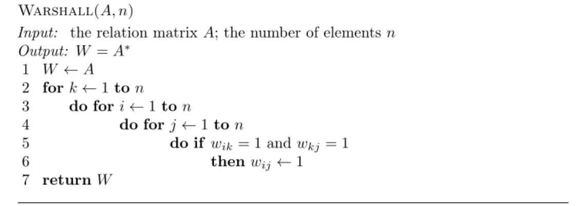
The transitive closure of a relation can be computed easily by the Warshall’s algorithm [2, 14]:

Warshall(𝐴, 𝑛)

Input: the relation matrix𝐴; the number of elements𝑛 Output: 𝑊 =𝐴^*

1 𝑊 ←𝐴 2 for𝑘←1to𝑛 3 do for𝑖←1to𝑛

4 do for𝑗←1to𝑛

5 do if 𝑤𝑖𝑘= 1 and𝑤𝑘𝑗= 1

6 then𝑤𝑖𝑗 ←1

7 return𝑊

Listing 1. Warshall’s algorithm.

The complexity of this algorithm isΘ(𝑛³).

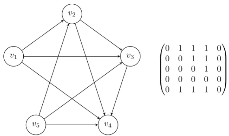
A binary relation can be represented by a directed graph (i.e. digraph) too. The relation matrix is equal to the adjacency matrix of the corresponding graph. See Fig. 1 for an example. Fig. 2 represents the graph of the corresponding transitive closure relation.

𝑣3

𝑣2

𝑣1

𝑣5 𝑣4

⎛

⎜⎜

⎝

0 1 0 0 0 0 0 1 1 0 0 0 0 1 0 0 0 0 0 0 0 1 0 0 0

⎞

⎟⎟

⎠

Figure 1. A binary relation represented by a graph with the corresponding adjacency matrix.

(20)

𝑣3

𝑣2

𝑣1

𝑣5 𝑣4

⎛

⎜⎜

⎝

0 1 1 1 0 0 0 1 1 0 0 0 0 1 0 0 0 0 0 0 0 1 1 1 0

⎞

⎟⎟

⎠

Figure 2. The transitive closure of the relation in Fig. 1.

2. Generalization of Warshall’s algorithm

Lines 5 and 6 in the Warshall’s algorithm presented in Listing 1 can be expressed as

𝑤𝑖𝑗←𝑤𝑖𝑗+𝑤𝑖𝑘·𝑤𝑘𝑗

using the operations defined above. If instead of the operations + and·we use two operations ⊕ and ⊙ from a semiring, a generalized Warshall’s algorithm results [11]:

Generalized-Warshall(𝐴, 𝑛)

Input: the relation matrix𝐴; the number of elements𝑛 Output: 𝑊 =𝐴^*

5 do𝑤𝑖𝑗 ←𝑤𝑖𝑗⊕(𝑤𝑖𝑘⊙𝑤𝑘𝑗) 6 return𝑊

Listing 2. The generalized Warshall’s algorithm.

The complexity of this algorithm is alsoΘ(𝑛³). This generalization leads us to a number of interesting applications.

(21)

3. Applications

3.1. Distances between vertices. Floyd–Warshall algorithm

Given a (di)graph with positive or negative edge weights (but with no negative cycles) and its modified adjacency matrix 𝐷0 = (𝑑⁰_𝑖𝑗), we can obtain the distance matrix𝐷 = (𝑑𝑖𝑗) in which𝑑𝑖𝑗 represents the distance between vertices 𝑣𝑖 and 𝑣𝑗. The distance between vertices𝑣𝑖 and𝑣𝑗 is the length of the shortest path between them. The modified adjacency matrix𝐷0= (𝑑⁰_𝑖𝑗)is the following:

𝑑⁰_𝑖𝑗=

⎧⎪

⎨

⎪⎩

0, if𝑖=𝑗,

∞, if there is no edge from vertex𝑣𝑖 to vertex𝑣𝑗, 𝑖̸=𝑗, 𝑤𝑖𝑗, the weight of the edge from𝑣𝑖 to𝑣𝑗, 𝑖̸=𝑗.

Choosing for ⊕theminoperation (minimum of two real numbers), and for ⊙the real addition (+), we obtain the well-known Floyd–Warshall algorithm as a special case of the generalized Warshall’s algorithm [5, 11, 12] :

Floyd-Warshall(𝐷0, 𝑛)

Input: the adjacency matrix 𝐷0; the number of elements𝑛 Output: the distance matrix𝐷

1 𝐷←𝐷0

2 for𝑘←1to𝑛 3 do for𝑖←1to𝑛

5 do𝑑𝑖𝑗 ←min{𝑑𝑖𝑗, 𝑑𝑖𝑘+𝑑𝑘𝑗} 6 return𝐷

Listing 3. Floyd-Warshall algorithm.

An example is presented in Fig. 3. The shortest paths can also be easily obtained by storing the previous vertex 𝑣𝑘 on the path, in line 5 of Listing 3. In the case of acyclic digraphs, the algorithm can be easily modified to obtain the longest distances between vertices and consequently the longest paths.

3.2. Number of paths in acyclic digraphs

Here, by path we understand a directed path. In an acyclic digraph the following algorithm counts the number of paths between vertices [4, 9]. The operation⊕,⊙ are the classical add and multiply operations for real numbers and let 𝑤𝑖𝑗 denote the number of paths from vertex𝑣𝑖 to vertex𝑣𝑗.

(22)

𝑣1 𝑣2 𝑣3

𝑣4

𝑣5

1 1

3

8 1

2 4 5

𝐷0=

⎛

⎜⎜

⎝

0 1 3 ∞ 8

∞ 0 1 ∞ 5

∞ ∞ 0 1 ∞

∞ ∞ ∞ 0 2

∞ ∞ 4 ∞ 0

⎞

⎟⎟

⎠ 𝐷=

⎛

⎜⎜

⎝

0 1 2 3 5

∞ 0 1 2 4

∞ ∞ 0 1 3

∞ ∞ 6 0 2

∞ ∞ 4 5 0

⎞

⎟⎟

⎠ Figure 3. A weighted digraph with the corresponding matrices.

Warshall-Paths(𝐴, 𝑛)

Input: the adjacency matrix 𝐴; the number of elements𝑛 Output: 𝑊 with number of paths between vertices

5 do𝑤𝑖𝑗 ←𝑤𝑖𝑗+𝑤𝑖𝑘·𝑤𝑘𝑗

6 return𝑊

Listing 4. Finding the number of paths between vertices.

The proof is omitted, as it is very similar to the one given in [2] for the original Warshall’s algorithm.

An example can be seen in Fig. 4. For example between vertices𝑣1and𝑣3there are 3 paths: (𝑣1, 𝑣2, 𝑣3);(𝑣1, 𝑣2, 𝑣5, 𝑣3)and(𝑣1, 𝑣6, 𝑣5, 𝑣3).

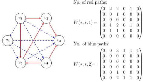
For the case when the arcs of the graph are colored, we may be interested in the number of monochromatic paths. The generalized algorithm can also be used for monochromatic subgraphs. The following novel algorithm (first described here) solves the problem for all colors at once.

In the adjacency (color) matrix,𝑎𝑖𝑗 is equal to the code of the color of the arc (𝑣𝑖, 𝑣𝑗), and is equal to 0, if there is no arc from𝑣𝑖 to𝑣𝑗. In the three-dimensional result matrix𝑊 the element𝑤𝑖𝑗𝑝represents the number of the paths from𝑣𝑖to𝑣𝑗

with𝑝-colored arcs each.

(23)

𝑣3

𝑣2

𝑣1

𝑣6

𝑣5

𝑣4

𝐴=

⎛

⎜⎜

⎝

0 1 0 1 0 1 0 0 1 0 1 0 0 0 0 1 0 0 0 0 0 0 0 0 0 0 1 0 0 0 0 0 0 0 1 0

⎞

⎟⎟

⎠

𝑊 =

⎛

⎜⎜

⎝

0 1 3 4 2 1 0 0 2 2 1 0 0 0 0 1 0 0 0 0 0 0 0 0 0 0 1 1 0 0 0 0 1 1 1 0

⎞

⎟⎟

⎠ Figure 4. An acyclic digraph and the corresponding matrices.

Warshall-Monochromatic-Paths(𝐴, 𝑛, 𝑐)

Input: adjacency color matrix𝐴; number of elements𝑛; number of colors 𝑐 Output: matrix𝑊 with number of monochromatic paths between vertices

1 Set all elements of𝑊 equal to0 2 for𝑖←1to𝑛

3 do for𝑗←1 to𝑛 4 do if 𝑎𝑖𝑗 ̸= 0

5 do𝑤𝑖𝑗𝑎𝑖𝑗 ←1

6 for𝑝←1to 𝑐

7 do for𝑘←1to𝑛 8 do for𝑖←1to𝑛

10 do𝑤𝑖𝑗𝑝←𝑤𝑖𝑗𝑝+𝑤𝑖𝑘𝑝·𝑤𝑘𝑗𝑝

11 return𝑊

Listing 5. Finding the number of monochromatic paths between vertices.

The sides for𝑝= 1, . . . , 𝑐of the three-dimensional matrix𝑊 contain the result for the different colors (see Fig. 5).

(24)

𝑣3

𝑣2

𝑣1

𝑣6

𝑣5 𝑣4

No. of red paths:

𝑊(*,*,1) =

⎛

⎜⎜

⎝

0 2 2 0 1 0 0 0 1 0 0 0 0 0 0 0 0 0 0 1 2 0 1 0 0 1 1 0 0 0 0 0 0 0 0 0

⎞

⎟⎟

⎠ No. of blue paths:

𝑊(*,*,2) =

⎛

⎜⎜

⎝

0 0 3 1 1 1 0 0 0 0 0 0 0 0 0 0 0 0 0 0 0 0 0 0 0 0 1 0 0 0 0 0 2 1 1 0

⎞

⎟⎟

⎠

Figure 5. An example of a colored digraph with the two sides of the solution matrix.

3.3. All paths in digraphs

The Warshall’s algorithm combined with the Latin square method can be used to obtain all paths in a (not necessarily acyclic) digraph [9]. A path will be denoted by a string formed by its vertices in their natural order in the path.

Let us consider a matrix𝒜 with the elements 𝐴𝑖𝑗 which are a set of strings.

Initially, the elements of this matrix are defined as:

𝐴𝑖𝑗 =

{︃{𝑣𝑖𝑣𝑗}, if∃ an arc from𝑣𝑖 to𝑣𝑗, 𝑖̸=𝑗,

∅, otherwise, for𝑖, 𝑗= 1,2, . . . , 𝑛. (3.1) If 𝒜 and ℬ are sets of strings, 𝒜ℬ will be formed by the set of concatenation of each string from𝒜with each string fromℬ, if they have no common letters:

𝒜ℬ={︀

𝑎𝑏⃒⃒𝑎∈ 𝒜, 𝑏∈ ℬ, if𝑎and𝑏 have no common letters}︀

. (3.2) If 𝑠 = 𝑠1𝑠2· · ·𝑠𝑝 is a string, let us denote by ^′𝑠 the string obtained from 𝑠 by eliminating the first character: ^′𝑠=𝑠2𝑠3· · ·𝑠𝑝. Let us denote by ^′𝐴𝑖𝑗 the set𝐴𝑖𝑗

in which we eliminate from each element the first character. In this case ^′𝒜is a matrix with elements^′𝐴𝑖𝑗.

Operations are: set union and set product defined as before.

Starting with the matrix𝒜defined as before, the algorithm to obtain all paths is the following, in which 𝑊𝑖𝑗 represents the set of paths from vertex𝑣𝑖 to𝑣𝑗.

(25)

Warshall-Latin(𝒜, 𝑛)

Input: the adjacency matrix 𝒜defined in (3.1); the number of elements 𝑛 Output: 𝒲 matrix of the paths between vertices

1 𝒲 ← 𝒜 2 for𝑘←1to𝑛 3 do for𝑖←1to𝑛

5 do if 𝑊𝑖𝑘̸=∅and𝑊𝑘𝑗̸=∅

6 then𝑊𝑖𝑗 ←𝑊𝑖𝑗∪𝑊𝑖𝑘′𝑊𝑘𝑗

7 return𝒲

Listing 6. Algorithm for finding all paths in digraphs.

An example is presented in Fig. 6: here, for example, between vertices𝑣1 and 𝑣3

there are two paths: 𝑣1𝑣3and𝑣1𝑣2𝑣3.

𝑣1 𝑣2 𝑣3

𝑣4

𝑣5

𝒜=

⎛

⎜⎜

⎝

∅ {𝑣1𝑣2} {𝑣1𝑣3} ∅ {𝑣1𝑣5}

∅ ∅ {𝑣2𝑣3} ∅ ∅ {𝑣3𝑣1} ∅ ∅ ∅ ∅

∅ ∅ {𝑣4𝑣3} ∅ {𝑣4𝑣5}

∅ ∅ ∅ ∅ ∅

⎞

⎟⎟

⎠

𝒲 =

⎛

⎜⎜

⎝

∅ {𝑣1𝑣2} {𝑣1𝑣3, 𝑣1𝑣2𝑣3} ∅ {𝑣1𝑣5} {𝑣2𝑣3𝑣1} ∅ {𝑣2𝑣3} ∅ {𝑣2𝑣3𝑣1𝑣5}

{𝑣3𝑣1} {𝑣3𝑣1𝑣2} ∅ ∅ {𝑣3𝑣1𝑣5} {𝑣4𝑣3𝑣1} {𝑣4𝑣3𝑣1𝑣2} {𝑣4𝑣3} ∅ {𝑣4𝑣5}

∅ ∅ ∅ ∅ ∅

⎞

⎟⎟

⎠

Figure 6. An example of digraph for all paths problem with the corresponding matrices.

Although the algorithm is not polynomial (due to the𝑊𝑖𝑘′𝑊𝑘𝑗multiplication), the method can be used well in practice for many cases.

(26)

3.4. Scattered complexity for rainbow words

The application described in this subsection can be found in [9]. Let Σ be an alphabet,Σ^𝑛the set of all length-𝑛words overΣ,Σ^* the set of all finite word over Σ.

Definition 3.1. Let𝑛 and𝑠 be positive integers,𝑀 ⊆ {1,2, . . . , 𝑛−1}and 𝑢= 𝑥1𝑥2. . . 𝑥𝑛 ∈Σ^𝑛. An 𝑀-subword of length𝑠of 𝑢is defined as𝑣 =𝑥𝑖1𝑥𝑖2. . . 𝑥𝑖𝑠

where

𝑖1≥1,

𝑖𝑗+1−𝑖𝑗∈𝑀 for𝑗 = 1,2, . . . , 𝑠−1, 𝑖𝑠≤𝑛.

Definition 3.2. The number of𝑀-subwords of a word𝑢for a given set𝑀 is the scattered subword complexity, simply𝑀-complexity.

Examples. The word𝑎𝑏𝑐𝑑has 11{1,3}-subwords: 𝑎,𝑎𝑏,𝑎𝑏𝑐,𝑎𝑏𝑐𝑑,𝑎𝑑,𝑏,𝑏𝑐,𝑏𝑐𝑑, 𝑐,𝑐𝑑,𝑑. The{2,3 4,5}-subwords of the word 𝑎𝑏𝑐𝑑𝑒𝑓 are the following: 𝑎, 𝑎𝑐, 𝑎𝑑, 𝑎𝑒,𝑎𝑓,𝑎𝑐𝑒,𝑎𝑐𝑓,𝑎𝑑𝑓,𝑏,𝑏𝑑,𝑏𝑒,𝑏𝑓,𝑏𝑑𝑓,𝑐,𝑐𝑒,𝑐𝑓,𝑑,𝑑𝑓,𝑒,𝑓.

Words with different letters are calledrainbow words. The𝑀-complexity of a length-𝑛rainbow word does not depend on what letters it contains, and is denoted by𝐾(𝑛, 𝑀).

To compute the𝑀-complexity of a rainbow word of length𝑛we will use graph theoretical results. Let us consider the rainbow word 𝑎1𝑎2. . . 𝑎𝑛 and the corresponding digraph𝐺= (𝑉, 𝐸), with

𝑉 ={︀

𝑎1, 𝑎2, . . . , 𝑎𝑛

}︀, 𝐸={︀

(𝑎𝑖, 𝑎𝑗)|𝑗−𝑖∈𝑀, 𝑖= 1,2, . . . , 𝑛, 𝑗= 1,2, . . . , 𝑛}︀

. For𝑛= 6, 𝑀 ={2,3,4,5}see Fig. 7.

The adjacency matrix𝐴= (𝑎𝑖𝑗)𝑖=1,𝑛

𝑗=1,𝑛 of the graph is defined by:

𝑎𝑖𝑗 =

{︃1, if𝑗−𝑖∈𝑀,

0, otherwise, for 𝑖= 1,2, . . . , 𝑛, 𝑗= 1,2, . . . , 𝑛.

Because the graph has no directed cycles, the element in row𝑖and column𝑗in𝐴^𝑘 (where𝐴^𝑘 =𝐴^𝑘⁻¹𝐴, with𝐴¹=𝐴) will represent the number of length-𝑘directed paths from𝑎𝑖 to 𝑎𝑗. If𝐼 is the identity matrix (with elements equal to 1 only on the first diagonal, and 0 otherwise), let us define the matrix𝑅= (𝑟𝑖𝑗):

𝑅=𝐼+𝐴+𝐴²+· · ·+𝐴^𝑘, where 𝑘 < 𝑛, 𝐴^𝑘+1=𝑂 (the null matrix).

The𝑀-complexity of a rainbow word is then 𝐾(𝑛, 𝑀) =

∑︁𝑛 𝑖=1

∑︁𝑛 𝑗=1

𝑟𝑖𝑗.

(27)

𝑎1 𝑎2 𝑎3 𝑎4 𝑎5 𝑎6

Figure 7. Graph for {2,3,4,5}-subwords of the rainbow word of length 6.

Matrix𝑅can be better computed using theWarshall-Pathsalgorithm described in Listing 4, which gives a matrix𝑊, and therefore𝑅=𝐼+𝑊.

For example, let us consider the graph in Fig. 7. [9] The corresponding adjacency matrix is:

𝐴=

⎛

⎜⎜

⎝

0 0 1 1 1 1 0 0 0 1 1 1 0 0 0 0 1 1 0 0 0 0 0 1 0 0 0 0 0 0 0 0 0 0 0 0

⎞

⎟⎟

⎠ .

After applying theWarshall-Pathsalgorithm:

𝑊 =

⎛

⎜⎜

⎝

0 0 1 1 2 3 0 0 0 1 1 2 0 0 0 0 1 1 0 0 0 0 0 1 0 0 0 0 0 0 0 0 0 0 0 0

⎞

⎟⎟

⎠

, 𝑅=

⎛

⎜⎜

⎝

1 0 1 1 2 3 0 1 0 1 1 2 0 0 1 0 1 1 0 0 0 1 0 1 0 0 0 0 1 0 0 0 0 0 0 1

⎞

⎟⎟

⎠ and then𝐾(︀

6,{2,3,4,5})︀

= 20,the sum of elements in𝑅.

Remark 3.3. For this case theWarshall-Pathsalgorithm can be slightly modified: because of the specific form of the graph the lines 2 and 4 can also be written in the following form:

2for 𝑘←2 to𝑛−1 4do for 𝑗←𝑖+ 1 to 𝑛

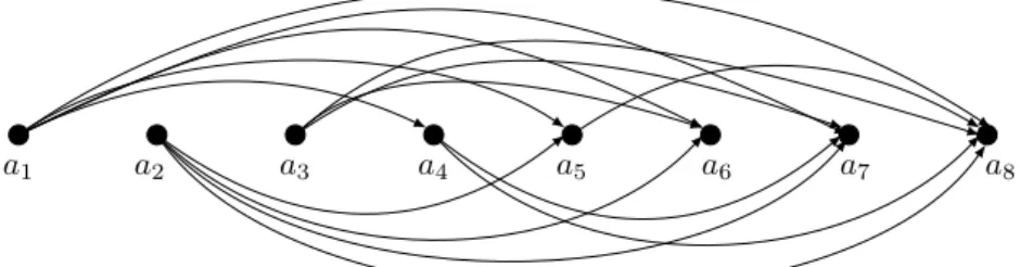
Using theWarshall-Latinalgorithm (Listing 6) we can obtain all nontrivial (with length at least 2)𝑀-subwords of a given length-𝑛rainbow word𝑎1𝑎2· · ·𝑎𝑛.

(28)

Let us consider a matrix 𝒜 with the elements 𝐴𝑖𝑗 which form a set of strings.

Initially this matrix is defined as:

𝐴𝑖𝑗 =

{︃{𝑎𝑖𝑎𝑗}, if𝑗−𝑖∈𝑀,

∅, otherwise, for 𝑖= 1,2, . . . , 𝑛, 𝑗= 1,2, . . . , 𝑛.

The set of nontrivial 𝑀-subwords is⋃︀

𝑖,𝑗∈{1,2,...,𝑛}𝑊𝑖𝑗.

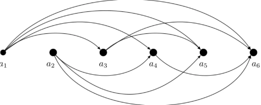
𝑎1 𝑎2 𝑎3 𝑎4 𝑎5 𝑎6 𝑎7 𝑎8

Figure 8. Graph for{3,4,5,6,7}-subwords of the rainbow word of length 8.

For𝑛= 8,𝑀={3,4,5,6,7}(see Fig. 8) the initial matrix is:

⎛

⎜⎜

⎝

∅ ∅ ∅ {𝑎1𝑎4} {𝑎1𝑎5} {𝑎1𝑎6} {𝑎1𝑎7} {𝑎1𝑎8}

∅ ∅ ∅ ∅ {𝑎2𝑎5} {𝑎2𝑎6} {𝑎2𝑎7} {𝑎2𝑎8}

∅ ∅ ∅ ∅ ∅ {𝑎3𝑎6} {𝑎3𝑎7} {𝑎3𝑎8}

∅ ∅ ∅ ∅ ∅ ∅ {𝑎4𝑎7} {𝑎4𝑎8}

∅ ∅ ∅ ∅ ∅ ∅ ∅ {𝑎5𝑎8}

∅ ∅ ∅ ∅ ∅ ∅ ∅ ∅

⎞

⎟⎟

⎠

The result of the algorithm in this case is:

⎛

⎜⎜

⎝

∅ ∅ ∅ {𝑎1𝑎4} {𝑎1𝑎5} {𝑎1𝑎6} {𝑎1𝑎7, 𝑎1𝑎4𝑎7} {𝑎1𝑎8, 𝑎1𝑎4𝑎8, 𝑎1𝑎5𝑎8}

∅ ∅ ∅ ∅ {𝑎2𝑎5} {𝑎2𝑎6} {𝑎2𝑎7} {𝑎2𝑎8, 𝑎2𝑎5𝑎8}

∅ ∅ ∅ ∅ ∅ {𝑎3𝑎6} {𝑎3𝑎7} {𝑎3𝑎8}

∅ ∅ ∅ ∅ ∅ ∅ {𝑎4𝑎7} {𝑎4𝑎8}

∅ ∅ ∅ ∅ ∅ ∅ ∅ {𝑎5𝑎8}

∅ ∅ ∅ ∅ ∅ ∅ ∅ ∅

⎞

⎟⎟

⎠ .

(29)

3.5. Special walks in finite automata

Let us consider a finite automaton 𝐴 = (𝑄,Σ, 𝛿,{𝑞1}, 𝐹), where𝑄 is a finite set of states, Σ the input alphabet, 𝛿: 𝑄×Σ → 𝑄 the transition function, 𝑞1 the initial state,𝐹 the set of final states. In the following, we omit to mark the initial and the final states. The transition function can also be generalized to words:

𝛿(𝑞, 𝑤𝑎) =𝛿(𝛿(𝑞, 𝑤), 𝑎), where 𝑞∈𝑄, 𝑎∈Σ, 𝑤∈Σ^*. A sequence of the form 𝑞1, 𝑎1, 𝑞2, 𝑎2, . . . , 𝑎_𝑛−1, 𝑞𝑛, 𝑛≥2,

where

𝛿(𝑞1, 𝑎1) =𝑞2, 𝛿(𝑞2, 𝑎2) =𝑞3, . . . , 𝛿(𝑞_𝑛−1, 𝑎_𝑛−1) =𝑞𝑛

is a walk in the automata labelled by the word 𝑎1𝑎2. . . 𝑎𝑛−1. This also can be written as:

𝑞1 𝑎1

−−−→𝑞2 𝑎2

−−−→𝑞3 𝑎3

−−−→ · · · −−−→^𝑎^𝑛⁻² 𝑞𝑛−1 𝑎𝑛−1

−−−→𝑞𝑛, or shortly: 𝑞1

𝑎1𝑎2...𝑎𝑛−1

−−−−−−→𝑞𝑛.

We are interested in finding walks with special labels: one-letter power words (power of a single letter) and rainbow words (containing only dissimilar letters).

3.5.1. Walks labeled with one-letter power words

For each pair𝑝, 𝑞of states we search for the letters𝑎for which there exists a natural 𝑘≥1such that we have the transition𝛿(𝑝, 𝑎^𝑘) =𝑞(see [11]). Let us denote these sets by:

𝑊𝑖𝑗 ={𝑎∈Σ| ∃𝑘≥1, 𝛿(𝑞𝑖, 𝑎^𝑘) =𝑞𝑗}, where𝑎^𝑘 is a length-𝑘one-letter power word.

Here the elements𝐴𝑖𝑗 of the adjacency matrix𝒜initially are defined as:

𝐴𝑖𝑗 ={𝑎|𝛿(𝑞𝑖, 𝑎) =𝑞𝑗}, for 𝑖, 𝑗= 1,2, . . . , 𝑛.

Instead of⊕we use here set union (∪) and instead of⊙set intersection (∩).

Warshall-Automata-1(𝒜, 𝑛)

Input: the adjacency matrix 𝒜; the number of states𝑛

Output: the matrix 𝒲 with sets of letters for one letter power words 1 𝒲 ← 𝒜

2 for𝑘←1to𝑛 3 do for𝑖←1to𝑛

5 do𝑊𝑖𝑗 ←𝑊𝑖𝑗∪(𝑊𝑖𝑘∩𝑊𝑘𝑗) 6 return𝒲

Listing 7. Finding walks labeled by one-letter power words.

(30)

𝑞1 𝑞2

𝑞3

𝑞4

𝑐

𝑏, 𝑑

𝑎 𝑏

𝑏 𝑏

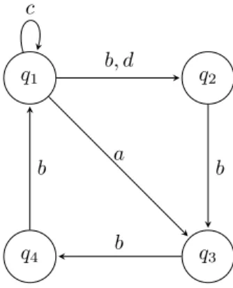
Figure 9. An example of a finite automaton without indicating the initial and final states.

The transition table of the finite automaton in Fig. 9 is:

𝛿 𝑎 𝑏 𝑐 𝑑

𝑞1 𝑞3 𝑞2 𝑞1 𝑞2

𝑞2 ∅ 𝑞3 ∅ ∅ 𝑞3 ∅ 𝑞4 ∅ ∅ 𝑞4 ∅ 𝑞1 ∅ ∅ Matrices for the graph in Fig. 9 are the following:

𝒜=

⎛

⎜⎜

⎝

{𝑐} {𝑏, 𝑑} {𝑎} ∅

∅ ∅ {𝑏} ∅

∅ ∅ ∅ {𝑏} {𝑏} ∅ ∅ ∅

⎞

⎟⎟

⎠, 𝒲=

⎛

⎜⎜

⎝

{𝑏, 𝑐} {𝑏, 𝑑} {𝑎, 𝑏} {𝑏} {𝑏} {𝑏} {𝑏} {𝑏} {𝑏} {𝑏} {𝑏} {𝑏} {𝑏} {𝑏} {𝑏} {𝑏}

⎞

⎟⎟

⎠.

For example𝛿(𝑞2, 𝑏𝑏) =𝑞4,𝛿(𝑞2, 𝑏𝑏𝑏) =𝑞1,𝛿(𝑞2, 𝑏𝑏𝑏𝑏) =𝑞2,𝛿(𝑞1, 𝑐^𝑘) =𝑞1for𝑘≥1.

3.5.2. Walks labeled with rainbow words

To find walks with rainbow labels, we can use the a variant of the Warshall- Latinalgorithm (Listing 6), where instead of string of vertices 𝑣1𝑣2· · ·𝑣𝑘 we use the corresponding string of labels of the edges(𝑣1, 𝑣2), . . . ,(𝑣𝑘−1, 𝑣𝑘).

Here the elements𝐴𝑖𝑗 of the adjacency matrix𝒜are initially defined as:

𝐴𝑖𝑗 ={𝑎|𝛿(𝑞𝑖, 𝑎) =𝑞𝑗}, for 𝑖, 𝑗= 1,2, . . . , 𝑛.

The concatenation𝑊𝑖𝑘𝑊𝑘𝑗 in the following algorithm is defined as in the formula (3.2). Each element of𝑊𝑖𝑘is concatenated with each element of𝑊𝑘𝑗only if these elements (which are strings) have no common letters. If a string appears more than once during concatenation, only one copy is retained. The following algorithm is a new one.

(31)

Warshall-Automata-2(𝒜, 𝑛)

Input: the adjacency matrix 𝒜; the number of states𝑛 Output: the matrix 𝒲 of the rainbow words between vertices

1 𝒲 ← 𝒜 2 for𝑘←1to𝑛 3 do for𝑖←1to𝑛

5 do if 𝑊𝑖𝑘̸=∅and𝑊𝑘𝑗̸=∅

6 then𝑊𝑖𝑗 ←𝑊𝑖𝑗∪𝑊𝑖𝑘𝑊𝑘𝑗

7 return𝒲

Listing 8. Finding walks labeled by rainbow words.

For the automaton in Fig. 9 the above algorithm uses the matrix𝒜:

𝒜=

⎛

⎜⎜

⎝

{𝑐} {𝑏, 𝑑} {𝑎} ∅

∅ ∅ {𝑏} ∅

∅ ∅ ∅ {𝑏} {𝑏} ∅ ∅ ∅

⎞

⎟⎟

⎠ and gives the following result:

𝒲=

⎛

⎜⎜

⎝

{𝑐} {𝑏, 𝑑, 𝑐𝑏, 𝑐𝑑} {𝑎, 𝑐𝑎, 𝑑𝑏, 𝑐𝑑𝑏} {𝑎𝑏, 𝑐𝑎𝑏}

∅ ∅ {𝑏} ∅

∅ ∅ ∅ {𝑏}

{𝑏, 𝑏𝑐} {𝑏𝑑, 𝑏𝑐𝑑} {𝑏𝑎, 𝑏𝑐𝑎} ∅

⎞

⎟⎟

⎠.

Conclusions

In 1962 S. Warshall published the algorithm later named after him for computing the transitive closure of a binary relation [14]. R. W. Floyd reported the application of this in the same year to determine the shortest paths in weighted graphs [5]. P. Robert and J. Ferland in their 1968 article [11] gave an interesting generalization that led to the applications discussed in this article [5, 9, 11, 12]. Two algorithms,Warshalł-Monochromatics-PathsandWarshall-Automata-2, are new applications firstly described here.

It is amazing how diverse the applications are. And there can be more!

Acknowledgements. The author thanks the anonymous reviewers for their at- tentive and thorough work in improving the paper with their helpful remarks.