Market liquidity and funding liquidity: Empirical analysis of liquidity fl ows using VAR framework
ADAM CZELLENG
1,2p1Faculty of Finance and Accountancy, Budapest Business School, Buzogany u. 10-12, Budapest, H-1149, Hungary
2GKI Economic Research Co., Budapest, Hungary
Received: August 20, 2018 • Revised manuscript received: February 10, 2019 • Accepted: March 31, 2019
© 2020 The Author(s)
ABSTRACT
One of the many consequences of financialization in the past decades has been the significant appreciation of the importance of financial markets’liquidity. In order to maintainfinancial stability, one must have a clear understanding of the sources of market liquidity (ML). Afiner comprehension of liquidity and its direction would help policy makers infine-tuning the current regulations while also identifying each of the elements that compose it. In this paper, a recursive vector autoregressive model is utilized to empirically analyze how to detect the causality relations between funding and ML in four post-communist countries (Czech Republic, Hungary, Slovakia and Poland). For the analyses freely accessible data on the balance sheets of aggregated banking sectors was utilized with the overall aim offinding a proxy for funding liquidity (FL) in every examined country. As a proxy for ML, government bonds’bid-ask spreads were utilized in the model. The paper provides an empirical evidence that FL drives ML in each economy. The results are clear, statistically significant and robust. They can be understood as evidence for the importance of the role of the trader’s FL for the liquidity offinancial assets’markets. The results of the paper have important implications for monetary policy, as well as micro- and macro-prudential regulation.
KEYWORDS
liquidity, vector autoregression,financial market,financial regulation JEL CLASSIFICATION INDICES
G10, G21, G28
pCorresponding author. E-mail: czelleng.adam@uni-bge.hu
1. INTRODUCTION
The recent emergence of a new monetary theory is not only the consequence of reaching the zero-lower bound and the need for new types of intervention by central banks, but also of the changes in the monetary transmission and of the emergence of new transmission channels.
One of the many significances of financialization in the past decades is how financial markets play an ever-increasing role not only in acquiring funds, but also in savings. The line between the activities of financial and non-financial organizations is constantly narrowing as non- financial organizations are equally providing credits, as well as managing financial portfolios and finance their operations by issuing bonds. Due to these, the importance of financial markets’ liquidity has appreciated, which made central banks to shift from their role of lenders of last resort to dealers of last resort (Mehrling 2014). This means that the central bank takes over the role of market maker when other actors in the market cannot or will not do it. During the times of crisis, it effectively entails stock purchases to help market par- ticipants’ balance sheet adjustments. It is especially important on the market of those products which serve as collateral during money market operations. From the perspective of the monetary policy what matters is the fact that the instruments’ liquidity influences the smooth functioning of the entirefinancial network, the amount of new investments and the balance sheets of all businesses. They equally influence the capacity and demand for credit and even the households’ wealth.
The literature distinguishes various types of liquidity, but in this study I focus only on two of them: funding liquidity (FL) and market liquidity (ML). FL describes a company’s or a bank’s ability to mobilize additionalfinancing to its operation quickly at the prevailing market price, while ML entails the pace at which a security can be traded in large volumes without signifi- cantly impacting the current price on the market. It goes without saying that these liquidity concepts are related to each other.
There is still no consensus among financial economists regarding the flow of liquidity and the relation between FL and ML.Gromb–Vayanos (2002), Brunnermeier–Pedersen (2006) and Mehrling (2014) argued that increasing FL would result in an elevated ML because financial institutions provide liquidity offinancial assets therefore their liquidity will impact the markets offinancial assets. On the other hand, the broad literature offinancialflexibility(a concept that emerged recently) considerfinancial markets’liquidity to determine the liquidity of the banking system and other companies. According to financial flexibility, a liquid financial market (i.e. a liquid financial asset) would provide liquidity to the banks as they would be able to easily raise funds by selling their assets, therefore they do not need to worry about the liability side of their balance sheets. According to the argument, ML implies easier portfolio allocation of the brokerage companies, mutual funds, and on the bond markets–the commercial banks, which helps them to react easier on their FL needs, hence they are able to hoard fewer liquid assets.
In order to maintain the financial stability, we need to understand the sources of ML.
Gaining a better comprehension on the drivers and directions of liquidity is not only necessary when financial markets unwind, but also during times of no turbulence in order to gain a sense of the vulnerabilities of system. A finer comprehension of the liquidity flow’s direction would allow policymakers tofine-tune the current regulation regime.
Empirical papers of the field focus on large, developed market economies, with special attention given to the USA. In the meantime, research on the components of ML on the emerging markets and open economies remains scarce. Empirically analyzing ML on small, open economies is inevitable because of the increasing financial integration. Small, open economies are integrated into the global financial system and global financial conditions have a growing impact on the domestic economic conditions in these countries. Changes in the global ML can directly lead to a change in ML on any national financial markets. On the other hand, changes in the global ML can lead to changes in the cost of financing thereby resulting in new conditions of FL therefore impacting ML. From the results it may be implied that due to globalization, the largest domestic financial market actors are also global actors. Therefore, if they are facing difficulties worldwide that can lead to a change in their way of conducting business locally within the domestic market environment.
In this paper, a recursive vector autoregressive model is utilized to empirically analyze the ways of detecting the causality relation between funding and ML of government securities in the cases of four small and open countries in Europe. The analyzed countries are the Czech Republic, Hungary, Poland and Slovakia–the Visegrad countries (V4).
2. LITERATURE REVIEW
Literature can divide into empirical and theoretical papers which analyze the determinants and sources of ML. Amihud – Mendelson (1980) managed to publish their seminal paper entitled Dealership Market – Market Making with Inventory. This study describes the behavior and profit maximizing conditions of a price setting monopolistic market maker. The study assumes that the market makers’inventory determines the market conditions for certain securities. Therefore, the paper describes the inventory dependent behavior of market makers by using number of assumptions. The conclusions of their model are that (i) market makers have a preferred inventory position which is aimed by the dealer’s pricing policy and (ii) market traders cannot make profit by using information which is also available for the market maker. It confirms Bagehot’s (1971) results that market makers trade with liquidity motivated traders.
O'Hara–Oldfield (1986)showed that a market maker’s bid-ask spread can be decomposed into a portion for the known limit orders, a risk-neutral adjustment for expected market orders, and a risk adjustment for market order and inventory value uncertainty. It is demonstrated that inventory has a pervasive role in affecting both the placement and size of the spread.
Treynor (1987) introduced the term of value-based investor who may be able to fulfill the dealer function, but at a significantly larger bid-asked spread than the market maker. Comparing to the value-based investor, the dealer has limited ability and willingness to absorb risk therefore the market maker has constraint regarding the position-long or short-he is willing to take. The value-based investors determine the price thus the dealer’s price is tied to the value-based investor’s price. The paper explains the asset prices by constant bid-ask spread based on their own liquidity and other risk exposures till the point the fundamental investors take the place of the market maker. According to Treynor, the larger the long market risk exposure of the market maker the higher the price will be; while the larger the short market risk exposure of market maker the lower the price will be.
Recently the causal relationship between FL and ML has received a lot of attention.Gromb– Vayanos (2002)in their frequently cited paper built a theoretical multiperiod model where some traders can trade with two identical riskyfinancial assets in segmented markets. In this case, the traders need to collateralize their positions separately in each market, which results infinancial constraints. Thefinancial constraints in the traders FL lead to an optimal level of liquidity being provided.
Brunnermeier–Pedersen (2006)provided a theoretical model which links assets’ML to the traders’FL. Theirfindings show that traders’ability to provide ML depends on the availability of the underlying funding, but the availability of their capital depends on the assets’ ML. Their model leads to understand that ML and FL are mutually reinforcing and leading to liquidity spirals.
Adrian – Shin (2009) empirically tested broker-dealers’ balance sheets and their role in providing liquidity. The paper argues that the availability of liquidity is significantly linked to the fluctuations in the leverage offinancial actors. The paper also states that the changes in dealers’ balance sheets can result changes in liquidity conditions therefore thefinancial intermediaries balance sheet can be used as macroeconomic variables to capture monetary policy framework.
ABank for International Settlements(BIS) paper, published in 2011, distinguishes two forms of liquidity –official and private liquidity. Official liquidity is defined as the unconditionally available form of liquidity provided by the central banks. While private liquidity is generated by the financial sector. The financial intermediaries provide ML to securities market for FL throughout interbank lending. There is an interaction between the above-mentioned liquidity categories. In normal times liquidity is generated by internationalfinancial actors while during financial turbulences liquidity is provided by the central banks. The paper outlines three major categories which are the drivers of liquidity. These are the (i) macroeconomic factors, (ii) other public sector policies, including financial regulation and (iii) financial factors. Jean-Pierre Landau (2013), who was the Chair of the Working Group which produced the above-quoted paper, also used the categories of private and public liquidity in his paper. The paper sum- marizes the behavior and interactions between the two components. “Global interactions be- tween private and official liquidity are both similar and different from those happening in domestic financial systems. I will argue that, depending on how they develop in the future, the shape of the internationalfinancial system could be very different: either moving toward more integration; or, following recent trends, introducing some progressive segmentation” (Landau 2013: 224).
Hedegaard (2011)empirically investigated the relation between the two liquidity categories by using time-varying margins on future contracts traded on the Chicago Mercantile Exchange (CME). The results showed that higher margins caused lower liquidity.
Jylha (2016)showed that FL causally affects ML by using an exogenous reduction in margin requirements. In 2005, the U.S. Securities and Exchange Commission (SEC) accepted a new methodology for margin requirements for index options but no changes were implemented for the margins of equity options. As an exogenous shock from market conditions affecting only a part of the market, the method was handled as a quasi-experiment allowing the identification of the causal link between FL and ML.
Just a few papers analyzed different dimensions of liquidity on the emerging markets and these papers mainly focused on equity markets. The International Organization of Securities Commissions (IOSCOs) summarized the responses of a survey about the source and
determinants of ML. The 21 countries (jurisdictions) responding to the questions mentioned four categories driving ML: (i) macro drivers; (ii) market microstructure; (iii) regulation; and (iv) products and services. As the paper says“Liquidity is becoming a critical issue in capital market development initiatives. As markets become global, an accompanying threat to small and less developed markets is the drying up of liquidity in domestic markets with a concurrent transfer of that liquidity to other major markets in the region”(IOSCO 2007: 8).
3. OUR RESEARCH METHOD
3.1. Data
The empirical analysis showed in this paper includes Visegrad countries. The group aims to advance their military, cultural, economic and energy cooperation with each other with strong financial market interdependencies. All four countries are members of the European Union and NATO. The leaders of Czechoslovakia, Hungary and Poland met in Visegrad, Hungary in 1991 to form the so-called Visegrad countries. The Visegrad countries have taken largely the same steps in an attempt to transform their economies in line with the capitalist economies of the West since the fall of the Soviet Union. This, as I argued, resulted in the emergence of a political-economic landscape in each country that made them to share a high degree of structural resemblance. However, there have also been fine differences. The aim of this paper is to detect the causality relation between different forms of liquidity in the Visegrad countries.
Measurement of liquidity has been a challenging issue as liquidity has various definitions and various characteristics. According to Tirole (2011), liquidity is a complex, multidimensional characteristic of thefinancial markets, hence a single statistic cannot describe this phenomenon well.
According to Lybek –Sarr (2002), liquidity measures can be classified into four groups, which are strongly related to the characteristics listed above. The classifications of liquidity measures are (i) transaction cost measures, (ii) volume-based measures, (iii) equilibrium price- based measures, and (iv) market impact measures.
The transaction cost measures can be further divided into explicit and implicit transaction cost. The former is related to every expense regarding a trade, including taxes, while the latter captures only the cost of execution. The most commonly used transaction cost measure is the bid-ask spread, which is known to capture almost all of the costs. If the transaction costs are lower, the investors prefer to trade with market makers, therefore lower transaction costs are associated with more liquid markets. Therefore, quarterly bid-ask spreads are applied in the model and it is generated as an average of daily bid-ask spread for each country. This is illustrated inFig. 1.
Measurement of FL is difficult. A common way to capture it is to use the TED spread, which is the spread between 3-month USD LIBOR and 3-month T-Bill (thus the cost of interbank funding over risk-free yields). However, the TED spread would be a sufficient proxy only for the US market.Jylha (2016) argues that TED spread would not even be acceptable for such an analysis.Drehmann–Nikolaou (2013)consider banks’bidding aggressiveness at the European Central Bank’s auctions as a good proxy.
This paper is built on the earlier work ofBrunnermeier et al. (2012) and Bai et al. (2017)in which balance sheet data were used to construct liquidity mismatch index to gauge the mismatch between asset and liability side. In this paper freely accessible data are utilized to gather information about the balance sheets of aggregated banking sectors in every analyzed country. As FL cannot be observed directly, the calculation of proxy variable is illustrated by Eq. (1).
funding liquidity proxy¼
liquid assets ratio
ði:e: cash; liquid securities; deposits at CBsÞ total assets
deposit ratio
ði:e: deposits; hortterm debtsÞ total liabilites
(1) The deposit ratio shows the proportion of deposits and short-term obligations for the banking system. The larger the ratio, the larger is the FL risk as the banking system faces a larger refinancing risk. This ratio can be viewed as an FL metrics. However, in order to maintain their financial flexibility banks may not fulfill their full credit capacity. They might call for more credit when they need to finance their growth or finance a bank run. That is why a ratio of deposit ratio and liquid assets ratio is applied. The liquid assets in proportion of the deposit ratio can demonstrate the extent to which financial institutions adjusted their asset side flexibility to their FL risk. The larger the FL proxy (liquid asset ratio/deposit ratio), the higher is the value of FL (or less the FL risk). The variable is very similar to the maturity mismatch calculations, which are commonly used to capture the FL risk of financial institutions (see BIS working papers of de Haan–van den End 2012;Bai 2015). AsFig. 2shows at the beginning of thefinancial crisis in 2007–2008, financial institutions faced with a drop in FL, and then, it was restored. It is important to mention that, because of the introduction of Basel 3, and thus, the Liquidity Fig. 1.Quarterly bid-ask spread for each country
Source: Reuters.
Coverage Ratio (2015) and Net Stable Funding Ratio (2018), the time series is not entirely homogeneous in terms of the systemic behavior.
Macro variables were also considered in the models based on the literature. GDP was considered as a main macro driver for markets as a proxy that is primary related to macro- economic performance. Chain link volume indexes, where 2005 is 100 for GDP, were collected for each country from Eurostat.
Harmonized Consumer Price Index was considered as a proxy for inflation. It measures the change over time in the prices of consumer goods and services which certainly contains important information regarding price stability therefore macroeconomic conditions regarding the countries. The source of the data was Eurostat as well.
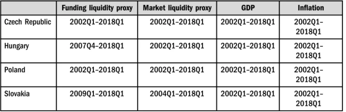
Overnight Index Swaps (OISs) were also included into the model in order to capture the cost of FL. OIS are financial instruments that allow financial institutions, intermediaries to swap interest rates and cash flows overnight to manage the liquidity positions. The data was collected from the countries’central banks. The data is summarized inTable 1.
Table 1.Data in details
Funding liquidity proxy Market liquidity proxy GDP Inflation Czech Republic 2002Q1–2018Q1 2002Q1–2018Q1 2002Q1–2018Q1 2002Q1– 2018Q1 Hungary 2007Q4–2018Q1 2002Q1–2018Q1 2002Q1–2018Q1 2002Q1–
2018Q1 Poland 2002Q1–2018Q1 2002Q1–2018Q1 2002Q1–2018Q1 2002Q1–
2018Q1 Slovakia 2009Q1–2018Q1 2004Q1–2018Q1 2002Q1–2018Q1 2002Q1–
2018Q1
Sources: Eurostat, Bloomberg and central banks.
2006Q1 2006Q3 2007Q1 2007Q3 2008Q1 2008Q3 2009Q1 2009Q3 2010Q1 2010Q3 2011Q1 2011Q3 2012Q1 2012Q3 2013Q1 2013Q3 2014Q1 2014Q3 2015Q1 2015Q3 2016Q1 2016Q3 2017Q1 2017Q3
Czech Hungary Poland Slovakia
Fig. 2.Time series of funding liquidity proxy for the analyzed countries Source: Author's calculation based on central banks data.
4. METHODOLOGY
In this paper, Vector Autoregressive (VAR) models are applied to capture the determinants and direction of liquidity in the sample countries. In the interest of structural impacts and changes, it is more convenient to detrend the data before fitting such models. Perhaps the most popular trend filter isHodrick–Prescott (1997)filter, or shortly, Hodrick-Prescottfilter (HP-filter). The famous methodology was originally developed to capture the cyclicality andfluctuations of US' real GDP, and therefore, assumed the output gap. The HP trend is extracted from a scalar time seriesxtusing a two-sided symmetric moving averagefilter. Given a time seriesx1,. . .,xT, the trend component τ1,. . .,τTis determined as the solution to the following minimization problem:
minfττgT
t¼1
XT
t¼1ðxtτtÞ2þλXTþ1
t¼2½ðτtþ1τtÞ ðτtτt1Þ2 (2) The objective is to minimize the variance of the cyclical componentct≡xtτtsubject to a penalty in the second difference ofτt, which measures the acceleration of the trend line. The parameterλcontrols the degree of smoothness of the trend component. In the limit, asλ→∞, the trend component will coincide with a linear deterministic trend. At the other extreme, for λ50,xt5τt. Hodrick and Prescott recommendλ51,600 for quarterly data so this is what was used to detrend the data in this paper as well.
The VAR models were designed to provide an alternative to the large macro-econometric models. In spite of the fact that the VAR models do not necessarily satisfy the Lucas’criteria for policy interventions, the methodology has become a widely used and popular technique in applied macroeconomic research. Sims (1980) introduced the methodology first in a famous paper, where he argued that empirical macroeconomic research should use small-scale models with less assumptions and with fewer constraints. Therefore, one of the method’s main ad- vantages is that the results are not an output of a black box but a relatively understandable and reliable model structure, hence the outputs can be interpreted with relative ease.
We can distinguish three types of VAR models: reduced, recursive and structural. In this paper, a recursive VAR model is introduced. In this type of model, the error terms in each regression equation are uncorrelated with the error in the preceding equations. As a result of this, some variables cannot realize the shocks in other variables simultaneously. Contempora- neous values as regressors can be considered to add. Therefore, the result of the equation system will depend on the order of the variables. This is called Cholesky decomposition so the variance- covariance matrix defining a diagonal matrix in which the elements on the main diagonal are equal to the standard deviation of the respective shock.
Withnnumber of variables, I would be able to buildn! number of recursive VAR models resulting in different equations, coefficients and residuals. In this paper, all countries’models include GDP, inflation, proxy for banking system FL and government securities bid-ask spread.1 Sousa–Zaghini (2004) andAcs (2013) argue that real variables like GDP adjust slowly that is why GDP is thefirst in the order. Inflation reacts quicker but still not as fast asfinancial var- iables, the banking sectors’reaction is fairly quick, while thefinancial markets react instantly.
1SeeBjornland (2000),Canova (995) and Uhlig (2005)for the technical details.
2 66 4
1 0 0 0
a21 1 0 0
a31 a32 1 0 a41 a42 a43 1 3 77 53
2 66 66 66 4
uGDPt uHICPt uFundingt
uMarkett 3 77 77 77 5
¼ 2 66 66 66 4
«GDPt
«HICPt
«Fundingt
«Markett
3 77 77 77 5
(3)
In an unrestricted VAR, I assume thatzt is a (n 3 1) vector of macroeconomic variables, which can be described as the following:
b0zt¼ gþb1zt−1þb2zt−2þ. . .þbpzt−pþut (4) wheregis a constant, biis a (n3n) matrix of coefficients anduiis a (n31) vector for the error terms, which has zero expected value and one unit of standard deviation with a covariance matrixΣ. A reduced form ofztcan be described like in Eq. (3).
zt¼ dþa1zt−1þa2zt−2þ. . .þapzt−pþet (5) where d¼ b−10 g; a1¼ b−10 bi and et ¼ b−10 ui are white noise processes with nonsingular covariance matrixU. The covariance matrix forut(Σ) is diagonal andb0has unity on its main diagonal.Ucan be estimated by using Ordinary Least Squares (OLS) method.
U¼covðetÞ ¼cov b−01ui
¼ b−01Σ b−010
(6) There aren(nþl)/2 distinct covariances (due to symmetry) inU. The assumption thatΣis diagonal and contains n elements implies that one needs n(n 1)/2 further restrictions to identify the system.
Based on the literature I identify three determinants of liquidity: (i) macroeconomic factors, (ii) financial factors and (iii) microstructure factors. Therefore, the following system of equa- tions was applied in the following order:
1. GDP,
2. inflation (Harmonised Indicies of Consumer Price (HICP)), 3. quarterly average bid-ask spread of the exchange,
4. quarterly average funding proxy variable, and 5. cost of FL (average OIS rate).
The impulse responses for the recursive VAR model have the same structure for every country.
4.1. Tests
Augmented Dickey-Fuller (ADF) unit root test was performed to assess the degree of integration of the variables. Applying ADF, we can identify whether the time series is stationary or not, which is a key underlying assumption for VAR methodology. I assume no autocorrelation among the error terms during the test to identify how many lags are supposed to apply. The data in this analysis was assessed to be non-stationary, therefore the appropriate variables were applied in the models.
The model describes the causal relationship between the selected variables that is why vector autoregressive models are highly sensitive to the length of lags involved. This means the number of lagged values, which are added to the system of equation, needs to be detected by an econometric method. The appropriate number of lags for the estimated VAR model has been decided based on the Akaike information criterion (AIC).2The widely used technique for model selection is a biased estimator.
AIC¼n
logσ2þ1
þ2p (7)
where p represents the number of parameters and σ2 represents the variance of the subsets model. Optimally that model should be considered, where the AIC (described by Eq. 1) is minimized. AIC is an asymptotically unbiased estimate. It is important to keep in mind that a relatively large lag length to the number of observations likely results in inefficient estimates of parameters or unstable models. While a too short lag length eventuates to misleading results as the causality structure remains unexplained.
Johansen’s cointegration test was also applied to confirm that the series are not cointegrated.
The test helps to ensure that the VAR is stable. In addition, I also use a residual correlation test to determine whether the residuals are correlated.
5. EMPIRICAL RESULTS
The analyzed countries are small, open economies therefore I can empirically test how financial integration influences the liquidity of those financial systems. The Visegrad countries have taken largely the same steps to transform their economies in line with the Western market economies after 1989. This resulted in the emergence of a political-economic landscape that led them to share a high degree of structural resemblance. However, there have also been a number of differences during this period of transformation, which from the perspective of this paper proved to have a special relevance. They help to explain to some extent the dissimilar results that the models provided.
In the 90s, Hungary was considered as one of the champions of the capitalist transformation by many observers. The country implemented market reforms that went beyond any of its neighbours’pace of transformation. However, soon after joining the EU the country became the sick man of the region. From 2002 onwards, the state began to extend its welfare programs far beyond its means, while also substantially cutting taxes. This combination of policies is what some later referred to as“fiscal alcoholism”. This went against the cyclical needs of the country’s economy as GDP growth was relatively high during the period that preceded it, reaching 3–4%
annually (Kiraly 2018).
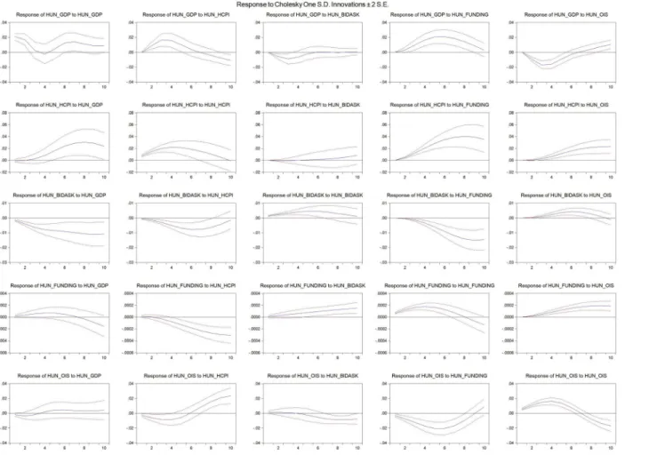
Results of the Hungarian VAR model is shown inFig. 1in the Appendix. In the case of Hungary, a shock in GDP has an effect on the harmonized consumer price index (HCPI).
HCPI is a widely used proxy to measure inflation. An increase in inflation for a GDP shock is understandable and expected because higher demand would lead to higher prices. The reverse effect is not clear however an unexpected rise in inflation can have an impact on
2The econometric technique was developed byAkaike (1974).
production becausefirms which already set their contracts for the period–and hence their costs – can realize higher revenue and profit by increasing their production. The bid-ask spread, which is used as a proxy for ML, also has a significant impact on GDP shocks as ML increases. A shock in inflation results in a significant jump in overnight swap prices just as expected.
From the perspective of the liquidity direction, both ways are significant thus it can be argued that ML has an impact on FL while FL has an impact on ML, however the latter’s influence is clearer and more significant. Therefore, we can clearly detect the inventory effect on ML.
Unexpected results emerged from the impulse functions for OIS shocks. According to the result of the VAR model based on the Hungarian data, a shock in the funding cost leads to a rise in inflation and results in better liquidity positions for financial intermediaries (while causes worse ML in par- allel). This can be a sign for a phenomenon called the“cost channel”, when due to the structure of firms’credits, higher interest rates makefirms to increase their prices, hence create inflation.
Polandfollowed a starkly differentfiscal and monetary path compared to Hungary before the crisis. During the years leading up to 2008, Poland and the Czech Republic had the lowest rate of credit inflows among the Central and Eastern Europe (CEE) countries. Following the outbreak of the 2008 subprime crisis, the country turned to the International Monetary Fund (IMF) for a one-year flexible credit line arrangement, that it was dully provided with, due to its healthy public debt position. This allowed for the country to maintain confidence in the eyes of foreign investors and put an end to further depreciation of the exchange rate. Domestic demand grew even in 2009 by 2% and remained positive later as well, which was partly due to the govern- ment’s counter-cyclical measures, primarily tax cuts. Additionally, with the inflow of EU funds and the necessary investments for the Euro 2012 football championship, Poland ended up being the only country to avert a recession in the whole of the EU after 2008.
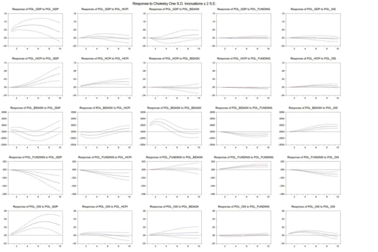
Results of the Poland VAR model are highlighted in Fig. 2of the Appendix. Many simi- larities can be detected in the results. An unexpected boom in economic growth points to higher inflation, and thus, higher overnight interest rates. However, FL decreases for economic growth shock. As Poland focused on domestic sources for economic growth, we can infer that increasing GDP implies an increase in investment willingness, which does not necessarily provide liquid assets to the banking system. According to the VAR model, the balance sheets of financial intermediaries have significant impact on the ML, while changes in bid-ask spread have no significant impact at all on the liquidity positions offinancial corporations. Contrary to the Hungarian results, the VAR model for Poland serves outcome in line with the expectations for a FL shock. This type of event produces higher bid-ask spread (thus lower ML) and reduced funding position forfinancialfirms.
Slovakia’s experience of transition differed somewhat from the aforementioned Eastern European countries. Breaking free and becoming a sovereign nation only in 1992, the country based their initial transformation primarily on domestic rather than international capital. Due to the resulting lack of incoming Foreign Direct Investment (FDI), the government had to borrow heavily and in less thanfive years it more than doubled its debt to GDP level from 21% in 1995 to almost 50% by 2000. Due to the increased pressure the government decided to open its borders to foreign capital and in the 2000s a great deal of the incoming capital was utilized for the reduction of the state debt, which allowed its debt to GDP level to return to 28% by 2008 and
with other macro indicators of the country showing similarly positive results. Slovakia was allowed to introduce the Euro by 2009.
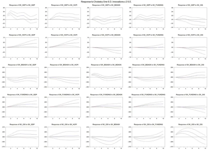
Results of the Slovakian VAR model are shown inFig. 3of the Appendix. An unexpected shock to GDP, inflation and interest rates (thus cost of funding) increases while ML hikes as well due to decreasing bid-ask spread. However, FL has a contradictory reaction as it increases for economic growth shock. The VAR model based on the detrended Slovakian data, the balance sheets offinancial intermediaries have significant impact on ML, while not statistically signif- icant link from the other way. In contrast with the Hungarian results but in line with Poland’s, a shock in the overnight interest rates generates a higher bid-ask spread (thus lower ML) and reduced funding position forfinancial firms.
In hindsight,Czech Republiccan be considered to have done the best overall of the Visegrad countries based on its macro indicators. The country had the best debt/GDP ratio from the outset already in the 1990s, reaching only 11.6% in 1995 and while going through a steady rise in the decade that followed, it still remained the lowest of the four countries before the crisis in 2008 (a mere 28.4%)
Results of the Czech VAR model are highlighted in Fig. 4of the Appendix. The impulse functions are similar to the previous findings; however, inflation has contradictory results. A shock in GDP results in a decrease in the inflation and an increase in the inflation results in a decreased interest rate. Overall, the direction of liquidity is statistically significant from the financial intermediaries to ML. However, in the case of Czech Republic a shock in the funding cost has significant direct impact on FL, yet no significant direct link to ML.
6. CONCLUSION
This paper empirically tested the source of liquidity in small, open economies. The results were somewhat contradictory in a few cases, yet overall, the following can be inferred. ML can be positively affected by economic growth and inflation, while negatively affected by an increase in the cost of funding. This is because the source of ML is the balance sheet of financial intermediaries.
This paper provides an empirical evidence that FL drives ML. The results are clear, signif- icant, robust and supported by the theoretical models. However, many researchers studied the topic, but just a few focused on the emerging markets. The results can be seen as a strong evidence for the important role of trader’s FL for the liquidity of financial assets’ markets in small, open economies as well.
The results of the paper have three key implications for practitioners related to central bank policy and commonality in liquidity. Due to financialization, financial markets play an ever- increasing role not only in acquiring funds, but the instruments’ liquidity has an effect on the smooth working of thefinancial network and has an impact on investments, the balance sheets of the businesses, moreover through the balance sheets they also influence the capacity and demand of credit or even the households’ wealth. The results infer that central banks can indirectly increase the asset’s liquidity by boosting the funding of dealers.
Due to financial integration and globalization, small and open economies do not appear to have efficient sovereign monetary policy according to many economists. Based on the empirical results, however these countries have strict limitations when applying monetary policy but central banks can nevertheless impact the financial markets’liquidity–the paper has not tested
the small and open economies independence when applying those monetary policy tools.
Maintaining the liquidity offinancial markets is a key element of the current regulation system.
Thefindings in this paper confirm that maintaining or even boosting the liquidity of the dealers can have a positive effect on thefinancial market’s liquidity.
ACKNOWLEDGMENT
The project has been supported by the European Union, co-financed by the European Social Fund and the budget of Hungary (Grant No. EFOP-3.6.2-16-2017-00007), titled“Aspects on the development of intelligent, sustainable and inclusive society: social, technological, innovation networks in employment and digital economy”.
REFERENCES
Acs, A. (2013): A Likviditases a realgazdasag kapcsolata az Egyes€ult Allamok p eldajan (Correalation of Liquidity and Economy on the Example of the US). Phd Thesis, Hungary: University of Szeged.
Adrian, T.–Shin, S. H. (2009):Money, Liquidity and Monetary Policy. Federal Reserve Bank of New York, Staff Report, No. 360.
Akaike, H. (1974): A New Look at the Statistical Model Identification. IEEE Transaction on Automatic Control, 19(6): 716–723.
Amihud, Y. – Mendelson, H. (1980): Dealership Market: Market-Making with Inventory. Journal of Financial Economics, 8(1): 31–53.
Bagehot, W. (1971): The Only Game in Town.Financial Analysts Journal, March–April, 12–14.
Bai, J.–Krishnamurthy, A.–Weymuller, C. (2017): Measuring Liquidity Mismatch in the Banking Sector.
The Journal of Finance, 73(1): 51–93.
BIS (2011):Global Liquidity–Concept, Measurement and Policy Implications. BIS CGFS Publications, No.
45, November.
Bjornland, H. C. (2000): Detrending Methods and Stylized Facts of Business Cycles in Norway–An In- ternational Comparison.Empirical Economics, 25(3): 369–392.
Brunnermeier, M. K.–Pedersen, H. L. (2009): Market Liquidity and Funding Liquidity.Review of Financial Studies, 22(6): 2201–2238.
Brunnermeier, M. K.–Corton, G.–Krishnamurthy, A. (2012): Risk Topography.NBER Macroeconomics Annual, No. 26.
Canova, F. (1995): The Economics of VAR Models. In: Hoover, K. (ed.):Macroeconometrics: Tensions and Prospects. New York: Kluwer Press, pp. 57–98.
Drehmann, M.–Nikolaou, K. (2013): Funding Liquidity Risk: Definition and Measurement. Journal of Banking and Finance, 37(7): 2173–2182.
Gromb, D.–Vayanos, D. (2002): Equilibrium and Welfare in Markets with Financially Constrained Ar- bitrageurs.Journal of Financial Economics, 66: 361–407.
Hedegaard, E. (2011):How Margins are Set and Affect Asset Prices. Working Paper, New York: University Leonard N. Stern School of Business, November.
Hodrick, R. J.–Prescott, E. C. (1997): Postwar US Business Cycle: An Empirical Investigation.Journal of Money, Credit and Banking, 29(1): 1–16.
IOSCO (2007):Factors Influencing Liquidity in Emerging Markets. Report of the IOSCO Emerging Markets Committee.
Jylha, P (2017): Does Funding Liquidity Cause Market Liquidity? Evidence from a Quasi-Experiment.
Working Paper, London: Imperial College, Business School.
Kiraly, J. (2018): Pieces of a Puzzle (A Concise Monetary History of the Hungarian Financial Crisis 2008).
Acta Oeconomica, 68(S): 143–163.
Landau, J. P. (2013): Global Liquidity: Public and Private. Economic Policy Symposium, Jackson Hole, Proceedings, pp. 213–259.
Lybek, T.–Sarr, A. (2002):Measuring Liquidity in Financial Markets. IMF.
Mehrling, P. (2014):Why Central Banking Should be Re-Imagined. BIS Papers, No 79.
O’Hara, M. – Oldfield, G. (1986): The Microeconomics of Market Making. Journal of Financial and Quantitative Analysis, 21(4): 361–376.
Sims, C. A. (1980): Macroeconomics and Reality.Econometrica, 48(1): 1–48.
Sousa, J.–Zaghini, A. (2004):Monetary Policy Shocks in the Euro Area and Global Liquidity Spillovers.
Working Paper, No. 309, European Central Bank.
Tirole, J. (2011): Illiquidity and All its Friends.Journal of Economic Literature, 49(2): 287–325.
Treynor, J. (1987): The Economics of the Dealer Function.Financial Analysts Journal, 43(6): 27–34.
Uhlig, H. (2005): What are the Effects of Monetary Policy? Results from an Agnostic Identification Pro- cedure.Journal of Monetary Economics, 52(2): 381–419.
Fig. 1.Results of VAR model based on Hungarian data.
Source:Author's own calculation.
mica70(2020)4,513–530527
Fig. 2.Results of VAR model based on Poland data.
Source: Author's own calculation.
ActaOeconomica70(2020)4,513–530
Fig. 3.Results of VAR model based on Slovakian data.
Source: Author's own calculation.
mica70(2020)4,513–530529
Open Access. This is an open-access article distributed under the terms of the Creative Commons Attribution 4.0 International License (https://creativecommons.org/licenses/by/4.0/), which permits unrestricted use, distribution, and reproduction in any medium, provided the original author and source are credited, a link to the CC License is provided, and changes–if any–are indicated. (SID_1)
Fig.4.ResultsofVARmodelbasedonCzechdata. Source:Author'sowncalculation.